Isolated Oscilloscope Inputs vs. Isolated Oscilloscope Probes

Some users in high-voltage test environments seek measuring instruments with isolated inputs because they want the safety and convenience of isolation without having to spend money on an isolated oscilloscope probe, like the Teledyne LeCroy DL-ISO or the Tektronix IsoVu®. While that's understandable, isolated inputs built into the instrument channel may be convenient, but they don't necessarily give you good performance, certainly not as good as  you would get from a high quality, high-voltage isolated probe.

Figure 1. Cascaded H-bridge signals captured using an isolated input (left) and an isolated probe (right).

Oscilloscope Basics: Cal Out and Aux Out

Fig. 1: Cal Out and Aux Out 
provide many useful outputs.

Oscilloscopes are generally thought of in terms of the signals that are input to them, but even oscilloscopes that are not equipped with function/signal generators can usually output some useful test signals.

Nearly all oscilloscopes have a Cal Out (calibration output) terminal on the front. Most Teledyne LeCroy oscilloscopes also have an Aux Out (auxiliary output) connector on either the front or back, depending on  model. Both outputs provide configurable signals that can assist you to compensate probes and attenuators, test frequency response, trigger waveform acquisition and coordinate multiple test instruments.

Four Essential Oscilloscope Network Security Practices

 Currently manufactured Teledyne LeCroy oscilloscopes utilize either the 64-bit Microsoft® Windows® 10 Professional or 32-bit Microsoft CE platforms to support the oscilloscope application. From a networking perspective, they are for all intents and purposes Personal Computers (PCs).

Using a commonly available computer operating system such as Microsoft Windows on a Teledyne LeCroy oscilloscope offers a multitude of advantages, such as the ability to link third-party software to oscilloscope operations and to connect to a wide variety of hardware. The downside of using a common operating system is the threat of malware. 

Malware (including but not limited to viruses, Trojan horses, worms, bots, keyloggers and spyware) can infect a PC via many paths. Examples include websites, USB memory sticks, emails and your local area network. Simply connecting an unprotected PC (i.e., unprotected Windows-based oscilloscope) to a “compromised” network is enough to infect the PC within seconds. Likewise, a compromised oscilloscope can infect an entire network.

Below, we list four practices Teledyne LeCroy strongly encourages all users to follow to minimize the risks that malware presents. Remember, the time you spend attending to oscilloscope network security is minimal compared to the cost of having to clean up an infected instrument. . .or network!

Oscilloscope Basics: External, Line and Fast Edge "Triggers"

An oscilloscope trigger synchronizes the oscilloscope timebase to the input signal so that the displayed trace is stable. In digital storage oscilloscopes, while the digitizer runs continuously converting analog voltage/current inputs to digital values, it is the trigger event that defines the “acquisition window,” marking the point where data is stored to acquisition memory, locking the signal data for display, measurement and further processing. 

Figure 1: The trigger setup showing the possible choices for the trigger source.

Triggers are set to fire based on the state of a trigger source waveform. What are commonly known as External, Line and Fast Edge "triggers" are not really different trigger types, per se, but alternative trigger sources.  Figure 1 shows the typical setup options for an Edge trigger, the most commonly used trigger type.  With Edge triggering, the oscilloscope is triggered when the source waveform crosses a user-defined threshold level and slope.  Usually, the source will be analog input channel C1-Cn. However, three other sources can be used to initiate an Edge trigger: an Ext(ernal) input, the Line (mains) power and, on some oscilloscopes, the built-in Fast Edge signal. 

Setting Up Your Oscilloscope for EFT Testing

Figure 1: The typical EFT test signal consists of
multiple exponential pulses arranged as pulse bursts.

A third type of electromagnetic compatibility (EMC) testing deals with how devices respond to electrical fast transients (EFT). EFTs are a series of fast, high frequency pulses, often occurring in bursts. These transient events are the result of electrical arcing. EFT pulse bursts occur when a power connection is made or broken, equipment is powered down or circuit breakers are switched. They also occur when inductive loads such as relays, switch contactors or heavy-duty motors produce bursts of narrow high-frequency transients on the power distribution system when de-energized.

The typical compound waveform used for EFT testing is shown in Figure 1.

Figure 2: Acquisition of two EFT bursts at
1.25 GS/s, zoomed to show several timing epochs.

The pulse waveform for EFT testing is defined by a risetime of 5 ns and a pulse width of 50 ns. These pulses are combined into bursts of 5 to 50 pulses spaced at from 10 to 100 µs (10 to 100 kHz). The bursts are typically spaced as much as 300 ms apart. Figure 2 shows an EFT test signal, with two EFT bursts captured by an oscilloscope on channel 2 sampled at 1.25 GS/s.

The two EFT pulse burst are shown in the upper left-hand trace (the two pink blocks). A series of zoom-on-zoom traces are opened to show several timing epochs. Trace Z2 (second from top left) shows a single burst. The zooms keep expanding the horizontal scale until finally at Z8 (bottom right) we see a single EFT pulse.

Following are six, important things to do to make sure you get the best EFT test measurements from your oscilloscope.

Setting Up Your Oscilloscope for Surge Testing

Figure 1: A typical EMC surge test waveform with
1.2 µs rise time and 50 µs half amplitude time.
Zoom trace Z1 shows the details of the rise time.
Click any image to expand it.

Electrical surges result from phenomena like lightning strikes and switching transients.  Electronic devices are subjected to simulated surges to confirm that they continue to operate properly following a surge, just as they are tested against electrostatic discharge. 

Surge pulses are similar to ESD pulses in that they have a very fast rise time, but the fall time is much, much slower. Figure 1 shows a typical surge pulse waveform. Surge testing involves similar measurements to those made for  ESD pulse testing—such as rise time, pulse width and max—but surge testing also requires some additional measurements, such as area under the pulse curve and transmitted charge. 

Figure 2: To verify the surge generator waveform, the
oscilloscope is connected to the generator through an attenuator.

As with ESD pulse tests, oscilloscopes are primarily used to “test the tester,” confirming the output of the surge generator. So, before a surge generator is hooked up to the device under test, it's required to hook it up to an oscilloscope and conduct a series of measurements to make sure the surge pulse is within specification. Figure 2 shows a typical surge test setup.

Following are three, important things to do to make sure you get the best surge measurements from your oscilloscope.

Setting Up Your Oscilloscope for ESD Pulse Testing

Figure 1: An ESD calibration test setup. 
The ESD gun discharges its waveform
into a properly attenuated current target. 

Electrostatic discharge (ESD) pulse tests are a type of conducted immunity testing done to confirm that a device can withstand a sudden transient electrostatic discharge. It is done by using an ESD gun to shoot a pulse of the required voltage at a device while testing that the DUT continues to operate properly. The ESD pulse shape simulates a person, carrying a static charge, touching a device. When their fingertip first touches the device, there is a leading edge with a high peak and fast decay, often visible in the real world as a spark flying from the fingertip. This is followed by a second edge due to the charge in the rest of the human body that propagates toward the fingertip with a time delay.

Oscilloscopes are most often used to “test the tester” in ESD pulse test setups, confirming that the pulse from the ESD gun is the right shape and meets the requirements of the standard to which the device is being tested. A typical calibration test setup is shown in Figure 1. The pulse from the ESD gun is fired directly into a current shunt target connected to the oscilloscope through an attenuator required to keep the signal within the limits of the oscilloscope’s 50 Ω input, which is used for this testing. Then, key parameters of the ESD pulse are measured per one of several standards, such as IEC 61000-4-2.  

ESD standards require a range of measurements. The most common are the initial edge 10% to 90% rise time, peak amplitude, pulse width, amplitude and current levels at specified times from the initial edge (e.g., T1 and T2), and time to half value. 

Following are four, important things to do to make sure you get the best ESD pulse measurements from your oscilloscope.

Oscilloscope Basics: When to Use Trend to Graph Oscilloscope Measurements

Figure 1: Applying the Trend operator to the
same input waveform illustrates how the
Trend is asynchronous to the input waveform.  

In a previous post, we described the characteristics of the Track math function and two key applications of using Tracks to graph oscilloscope measurement data: anomaly detection and waveform demodulation. In this post, we'll discuss the characteristics and uses of the Trend function.

To illustrate an important distinction between Tracks and Trends, the Trend math operator in Figure 1 is now applied to the same signal as was the Track in our previous post without first reacquiring the input waveform. 

Note that unlike a Track, the Trend is not time-synchronized to the input waveform. Only the order of events, and not the timing of events, is retained. The underlying shape of the Track may be displayed in the Trend because the same measurement values from a single acquisition are displayed in the same sequence—however, the timing information of when each of the values has occurred is not retained in the Trend. Therefore, unlike the Track, the Trend does not point to the location of an anomaly. Without time scaling, the Trend does not have the frequency information needed to demodulate an input waveform.

Oscilloscope Basics: When to Use Track to Graph Oscilloscope Measurements

Figure 1: Pulse Width Modulated waveform (yellow)
and Track math operator (blue),
where the X-axis scaling is identical for both.

Modern oscilloscopes contain many tools that can be used for analyzing data, including Track and Trend math functions. Both Tracks and Trends graphically display measurement results and locate anomalies. The main similarity between Tracks and Trends is that the Y-axis of both operators is the measurement parameter itself (for example, Pulse Width, Duty Cycle, Rise Time, Slew Rate, etc.). The main difference between the two math operators is their X-axis, in which the Track uses the identical X-axis and synchronous horizontal scaling as the input waveform, whereas the Trend uses units of chronology. A Track, in essence, is a waveform of the measurement values. A Trend is a data logger showing the history of change in measured parameter values, but points are not necessarily synchronous with the measured waveform.

Use Tracks for Anomaly Detection

The Track provides valuable debugging information by directly pointing to an area of interest. 

Notice the negative-going spike in the Track waveform in Figure 1. Figure 1 occurs at the point in time where the input waveform reaches its most narrow pulse width, and the Track instantly finds it, indicating when one measurement deviates from the others in the graph. The Track identifies the exact location in time where the narrowest or widest pulse width has occurred, and fully describes the measurement changes occurring throughout the entire waveform. Since oscilloscopes can acquire thousands or even millions of waveform edges within a single acquisition, the Track allows an engineer to quickly "find the needle in a haystack".

PCI Express 4.0 Error Detection Using a BERT and Oscilloscope

Figure 1: BERT and Oscilloscope connection
for PCI Express 4.0 error detection.

The PCI Express® 4.0 standard specification requires an oscilloscope with at least 25 GHz analog bandwidth and a BERT which can test bit rates of at least 16 Gbps. The BERT provides a known input pattern to the PCIe® device under test (DUT), and the DUT is instructed to regenerate the identical bit pattern while placed in loopback mode. Since a BERT can output a signal when a bit error is detected, this signal can be input to the oscilloscope to trigger a synchronized capture when an error occurs. By combining the capabilities of these two instruments, a powerful combination of real-time error detection and characterization can emerge.

Connecting the Instruments

In Figure 1, a known pattern is connected from the BERT PPG D1 output to the PCIe DUT input via a 2.92 mm K-type cable. The DUT attempts to regenerate the same data pattern, while the DUT output is routed to both the BERT error detector input and the oscilloscope channel 1 via 2.92 mm K-type tables and a power splitter. An error-free reference signal is connected between the BERT D2 output to the oscilloscope channel 2, along with the error trigger signal from the error detector output to the oscilloscope channel 3. An oscilloscope Edge trigger is set on the rising edge of the error detector output signal on C3.

Configuring Dynamic Oscilloscope Measurements Using Advanced Customization

Figure 1. The Advanced Customization option
lets you seamlessly and continuously update the
input of one parameter with the output of another.

With the installation of the Advanced Customization (XDEV) option on Teledyne LeCroy MAUI® oscilloscopes, you can create a measurement parameter whose input value is dynamically updated with each new trigger by the output value of another measurement parameter. All that is required is three simple lines of VBScript. 

To demonstrate, we’ll use the example of taking the x@max value measured on each acquisition and using it to dynamically populate the X position used by the measurement parameter lvl@x. However, these principles could be applied to any two parameters that share a logical/mathematical relationship, or to a parameter and a math function (for example, to use the output of a parameter as the multiplier for a Rescale function).

Transmission Lines for Oscilloscope Users, Part 4

Figure 1: Characteristic waveform when the source
impedance is lower than the cable impedance.

In Part 3, we saw the pattern of reflections that occur when both the source impedance and the oscilloscope input impedance are higher than that of the interconnect, and how those reflections affected the rise time measurement. Now let’s briefly consider what happens when the source impedance is lower than the impedance of the connecting cable. 

For this example, the source voltage is a 3.3 V square wave and the source impedance is 9 Ω. As before, our transmission line is a 50 Ω coaxial cable connecting the source to the oscilloscope. If the oscilloscope input termination is set to 1 MΩ, we see the interesting waveform shown in Figure 1.

Transmission Lines for Oscilloscope Users, Part 3

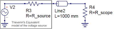
Figure 1: The Thevenin equivalent circuit model can be used
to characterize a voltage source with respect to the 
interconnect cable and oscilloscope input termination.

In Part 2, we demonstrated how to calculate the instantaneous impedance of a transmission line. However, any measurement made using an oscilloscope should consider not only the transmission line, but the source, the transmission line and the oscilloscope as a system. Therefore, characterizing your source, as well as knowing the effects of your oscilloscope input impedance, is important to developing the “situational awareness” needed to interpret measurements properly.

Two terms needed for us to characterize the source are the Thevenin source voltage and the Thevenin source resistance. Once we know these, we have all the pieces we need to fully understand what is happening with our measurements. This is true whether the signal source is a Cal terminal or a device-under-test.

Transmission Lines for Oscilloscope Users, Part 1

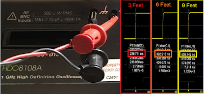
Figure 1: The rise time of the Cal signal seems to
increase significantly by increasing the length of the
interconnect cable. Is it true? Click image for details.

This post is the first of a series that will discuss what every oscilloscope user needs to know about transmission lines. It is going to introduce you to the absolutely most important signal integrity principles everybody needs to know when using an oscilloscope to measure signals with rise times shorter than 10 nanoseconds. After demonstrating some easily misinterpreted measurements, we’re going to look “under the hood” at what’s really happening to show you how it's all about the principles of transmission lines. Awhile back, Dr. Eric Bogatin offered a condensed version of What Every Oscilloscope User Needs to Know About Transmission Lines that summed up the key takeaways, but by revisiting “Transmission Lines 101” with us here, we’ll hopefully also show you a different way of thinking about your measurements.

How to Use Memory Properly

In a recent post, we addressed setting sample rate for serial data acquisition, but let’s look again at how time per division (time/div), memory length and sample rate all interact, and what you can do to optimize your use of oscilloscope capture memory when setting up your timebase.

Figure 1: Sample rate as a function of time/div for three different memory lengths.
Longer memory extends the range of time/div settings that support the highest sample rate.

TDME Primer: Selecting Sample Rate for Serial Bus Analysis

Figure 1. Sample rate of only four sample points per bit
decodes correctly and lengthens serial bus acquisition.

Teledyne LeCroy supports trigger, decode, measure/graph, and eye diagram (TDME) software options for over 20 serial data standards, and the list is growing. This series will address practical tips for using TDME software successfully, and showcase some examples of applying TDME capabilities to real-world problems.

Given the wide range of protocols supported, you might be curious about how to best choose the oscilloscope sampling rate for a given standard when acquiring serial data signals. The optimal sample rate is determined by three principal factors: 

1) the bandwidth of the signal being digitized by the oscilloscope’s analog-to-digital converter (ADC);

2) the desired duration of the acquisition;

3) what you are going to do with the acquisition.

Oscilloscope Basics: Multiplexed Front Panel Controls

Fig. 1. Modern,
slim front panel.

Most Teledyne LeCroy oscilloscopes are equipped with traditional front panel controls—knobs and buttons—that are a (literally) handy way to make basic acquisition settings such as gain, timebase and trigger level. While all these could be made using the oscilloscope software, using the front panel allows you to keep dialogs closed and more of the screen “real estate” available for viewing traces as you modify these settings.

In order to optimize that real estate, front panels have become increasingly slim, and many front panel controls on newer Teledyne  LeCroy oscilloscopes are multiplexed, meaning they have multiple functions or can be used to control multiple on-screen objects. Here is a list of tips to keep in mind when using the front panel.

A Real-World FFT Example

Figure 1: Shown at top right is the output of a
5V switch-mode power supply acquired
with an RP4030 active voltage-rail probe

Performing a fast Fourier transfer (FFT) on an oscilloscope can be likened to driving a car. Just as there are two dominant strains of power-train transmissions, there are two dominant approaches to transferring signals acquired on an oscilloscope from the time domain to the frequency domain. There's the stickshift approach, in which the FFT parameters are set manually, and the automatic approach, in which you let the oscilloscope make decisions for you.

Fast Fourier Transforms: Automatic Edition

Figure 1: Shown is the user interface for Teledyne LeCroy's
Spectrum Analyzer software option

Many motorists love the experience of driving a sporty car with its convertible top down and a stickshift manual transmission. Others don't want the hassle of a clutch and prefer the user-friendly feel of a slick automatic that does some of the work for them. Oscilloscopes can provide the same sort of choice for many measurement tasks in the same instrument.

The Resolution Revolution In Oscilloscopes

Figure 1: Teledyne LeCroy's WavePro HD exemplifies
today's high-resolution, high-bandwidth instruments

Oscilloscopes have been around for a very long time now, and older oscilloscope users will remember the heyday of those analog boat anchors of the '60s and '70s. Many have survived and are still usable if you don't need much bandwidth (and have the means to calibrate them if necessary). I used to scout local hamfests looking for bargains on them. Many techs and engineers cut their teeth on those behemoths. You could learn a lot about design if you poked around inside them, too.