You need to test, we're here to help.

You need to test, we're here to help.
Showing posts with label frequency domain. Show all posts

18 July 2022

Six Principles of FFT Analysis Using Real-time Oscilloscopes

Figure 1. A 100 MHz sine wave in the time domain and its spectrum in the frequency domain showing the one peak at 100 MHz.
Figure 1. A 100 MHz sine wave in the time domain
and its spectrum in the frequency domain showing
the one peak at 100 MHz. Click on any image to enlarge.
By Prof. Eric Bogatin,
Teledyne LeCroy Fellow

The following piece was published in Signal Integrity Journal and is excerpted here by permission of Signal Integrity Journal.

***************************

We live in the time domain. This is where we measure all digital performance. But sometimes, we can get to an answer faster by taking a detour through the frequency domain. With these six principles, we can understand how an oscilloscope transforms time domain measurements into a frequency domain view. All six principles are applied “under the hood” by oscilloscopes with a built-in FFT function. (Our note: Also by software packages designed for spectral analysis, such as the SPECTRUM-1 and SPECTRUM-PRO-2R options.)

1. The spectrum is a combination of sine wave components

In the frequency domain, the only waveforms we are allowed to consider are sine waves. There are other special waveforms combinations of which can describe any time-domain waveform, such as Legendre polynomials, Hermite polynomials or even wavelets. The reason we single out sine waves for a frequency domain description, is that sine waves are solutions to second order, linear, differential equations—the equations found so often in electrical circuits involving resistor, capacitor and inductor elements. This means signals that arise or have interacted with RLC circuits are described more simply when using combinations of sine waves than any other function because sine waves naturally occur. 

14 March 2022

WavePulser 40iX vs. Time Domain Reflectomer (TDR) or Vector Network Analyzer (VNA)

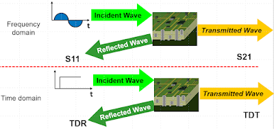
Figure 1: S-parameters and TDR responses are two means to the same end, characterizing interconnects.
Figure 1: S-parameters and TDR responses are two means to
the same end, characterizing interconnects.
Oscilloscopes are used to measure signals, usually as voltages vs. time, and signals come from active devices. But interconnects are passive structures that don’t produce their own signals. To characterize interconnects, you need a stimulus-response system.

There are two, principal types of stimulus-response systems used to characterize interconnects: Vector Network Analyzers (VNAs) used to measure S-parameters in the frequency domain, and Time Domain Reflectometers used to measure impulse responses in the time domain. Each uses a different type of incident signal and a different formalism, but as long as the interconnect is linear, passive and time invariant, both S-parameters and impulse responses yield the same information content in different formats and can be translated from one into another.

So, which do you need? We’ll look briefly at what each does and what are the criteria that might require you to have one versus the other.

21 February 2022

9 Important Things to Know When Making Sensitive Measurements with Oscilloscopes

We've routinely posted on how you can characterize your total measurement system to gain important "situational awareness" when using an oscilloscope to make sensitive measurements. The knowledge gained from these tests helps you properly interpret your measurement results so that you can deduce what is actually going on with your circuit, versus what is an artifact of the measurement system. Listed here are nine important things you should know before making sensitive measurements with your oscilloscope, with links to blog posts that instruct you how to test them.

08 April 2019

Fast Fourier Transforms: Automatic Edition

Figure 1: Shown is the user interface for Teledyne LeCroy's Spectrum Analyzer software option
Figure 1: Shown is the user interface for Teledyne LeCroy's
Spectrum Analyzer software option
Many motorists love the experience of driving a sporty car with its convertible top down and a stickshift manual transmission. Others don't want the hassle of a clutch and prefer the user-friendly feel of a slick automatic that does some of the work for them. Oscilloscopes can provide the same sort of choice for many measurement tasks in the same instrument.

02 April 2019

Fast Fourier Transforms: Stickshift Edition

Figure 1: Shown at left is a 50-kHz input sine wave with the FFT of the same signal at right
Figure 1: Shown at left is a 50-kHz input sine wave
with the FFT of the same signal at right
Perhaps you're old enough to remember when more cars had stickshifts. They're a little bit more work to drive than cars with automatic transmissions, but the experience can be much more rewarding. Oscilloscopes these days are like cars with both types of transmissions, and you can use either one for many tasks. One of those tasks is fast Fourier transforms (FFTs), and in this post we'll take you through driving an oscilloscope to perform an FFT with a stickshift.

22 February 2019

About Data Truncation in Fast Fourier Transforms

The first precondition of using the Fourier transform is a repetitive signal
Figure 1: The first precondition of using the Fourier transform
is a repetitive signal
Our last post discussed how time-domain signals acquired by an oscilloscope might be translated into the frequency domain using the discrete Fourier transform. We noted that using the Fourier transform only works if our signal is repetitive (Figure 1), and that it allows us to identify only harmonics of the first harmonic frequency, which is 1/acquisition window. Moreover, the discrete Fourier transform, if used on a large number of data points, is relatively slow to calculate.

30 January 2019

Getting From the Time Domain to the Frequency Domain

A fundamental underlying assumption of a discrete Fourier transform is a repetitive waveform
Figure 1: A fundamental underlying assumption of a discrete
Fourier transform is a repetitive waveform
Fundamentally, oscilloscopes are time-domain instruments: We use them to acquire signals from our circuitry or device under test, and the instrument displays them in the time domain. We see the voltage of the signal in the vertical axis, and we see how that voltage changes over time in the horizontal axis.

30 April 2018

Investigating IoT Wireless Signals (Part II)

This screen capture depicts frequency demodulation and subsequent Manchester decoding of the bit stream
Figure 1: This screen capture depicts frequency demodulation
and subsequent Manchester decoding of the bit stream
Internet of Things (IoT) devices must communicate with their peers--other IoT devices--as well as with the host system that governs their activities. In our previous post, we examined how to perform amplitude and frequency demodulation of RF bursts, such as Bluetooth Low Energy (BLE) advertising bursts. We'll continue with other methods of analyzing RF signals.

20 February 2018

Transmission Lines (Part I): Introduction

All oscilloscopes have a Cal output like the one pictured here
Figure 1: All oscilloscopes
have a Cal output like the
one pictured here
Somewhere on the front panel of almost any oscilloscope is a "Cal" reference signal output (Figure 1). That signal is really intended for adjusting the capacitance compensation screw to calibrate a 10X high-impedance probe, but most of us know it simply as the Cal signal. Have you ever noticed that the Cal signal's rise time seems to be highly dependent on the length of the cable attached to it, and maybe even wondered why?

17 December 2014

What S-parameters Reveal About Interconnects (Part III)

How ripple is introduced into S11 and S21
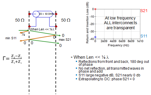
Figure 1: How ripple is introduced into S11 and S21
S-parameters are a great tool for understanding exactly what happens to a signal as it traverses an interconnect such as a transmission line. How much of it propagates through, and how much reflects off of impedance mismatches? From plotting return loss against insertion loss, we've weighed how much return loss may be tolerable before it significantly impacts insertion loss. Now we'll turn our attention to some common patterns exhibited by S11 and S21 and what they mean to the performance of an interconnect.

09 December 2014

What S-parameters Reveal About Interconnects (Part II)

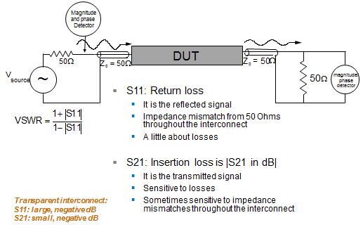
Measuring S-parameters of a two-port interconnect
Figure 1: Measuring S-parameters
of a two-port interconnect
Having previously covered some of the fundamentals of S-parameters, it's now time to dig a little deeper into what they can show us about an interconnect; say, for example, a two-port microstrip line on a PC board. Unlike the one-port DUT in our earlier post, this configuration gives us the opportunity to look at not only S11 (return loss or reflected signal), but also S21 (insertion loss or transmitted signal).

03 December 2014

What S-Parameters Reveal About Interconnects

S-parameters are derived by applying an incident wave to an interconnect
Figure 1: S-parameters are derived by applying an incident
wave to an interconnect; we can consider this process in either
the time or frequency domains
S-parameters are a popular means of characterizing an interconnect. By feeding the interconnect with a precision reference signal and measuring how much of that signal propagates through the connector and how much is reflected, we learn everything we need to know about its performance. This will be the first in a series of posts about the insights we can glean from S-parameters with practical examples of common measurement scenarios.

15 May 2014

Back to Basics: S-parameters

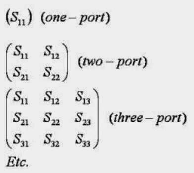
S-matrices for one-, two-, and three-port RF networks
Figure 1: S-matrices for one-, two-,
and three-port RF networks
Suppose you have an optical lens of some sort onto which you shine a light with a known photonic output. While most of the incident light passes through the lens, some fraction of the light is reflected and some is absorbed (the behavior is also dependent on the wavelength of the incident light). You'd like to characterize that lens: Exactly how much light was reflected? How much passed through? What is it about the lens that prevented all of the light from passing through?

25 September 2013

Back to Basics: What is an FFT?

An FFT of a 300-kHz square wave.
Figure 1: An FFT of a 300-kHz square wave.
In an earlier post, we discussed the basics of setting up a fast-Fourier transform (FFT) on an oscilloscope, and why you'd want to use an FFT to get a frequency-domain view of a time-domain signal in the first place. It might be a good idea to take a step back and dig into just what an FFT is (Figure 1).

30 August 2013

Oscilloscope Basics: Setting Up FFTs

Capture time determines the frequency resolution, Δf
Figure 1: Capture time determines the
frequency resolution, Δf.
For most of their history, oscilloscopes have been thought of chiefly as a time-domain instrument. That is, an oscilloscope facilitates the observation of changes in a signal's amplitude over time. However, many modern digital and mixed-signal oscilloscopes provide spectral analysis capabilities based on fast Fourier transforms (FFTs) that convert a time-domain waveform into the frequency domain. There are lots of good reasons for taking advantage of this capability. Perhaps the most important is to gain insight into characteristics of the signal that simply are not apparent from a time-domain perspective.