You need to test, we're here to help.

You need to test, we're here to help.
Showing posts with label transmission line. Show all posts

14 February 2022

Transmission Lines for Oscilloscope Users, Part 4

Figure 1: Characteristic waveform when the source impedance is lower than the cable impedance.
Figure 1: Characteristic waveform when the source
impedance is lower than the cable impedance.
In Part 3, we saw the pattern of reflections that occur when both the source impedance and the oscilloscope input impedance are higher than that of the interconnect, and how those reflections affected the rise time measurement. Now let’s briefly consider what happens when the source impedance is lower than the impedance of the connecting cable. 

For this example, the source voltage is a 3.3 V square wave and the source impedance is 9 Ω. As before, our transmission line is a 50 Ω coaxial cable connecting the source to the oscilloscope. If the oscilloscope input termination is set to 1 MΩ, we see the interesting waveform shown in Figure 1.

07 February 2022

Transmission Lines for Oscilloscope Users, Part 3

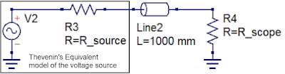
Figure 1: The Thevenin equivalent circuit model can be used to characterize a voltage source with respect to the  interconnect cable and oscilloscope input termination.
Figure 1: The Thevenin equivalent circuit model can be used
to characterize a voltage source with respect to the 
interconnect cable and oscilloscope input termination.
In Part 2, we demonstrated how to calculate the instantaneous impedance of a transmission line. However, any measurement made using an oscilloscope should consider not only the transmission line, but the source, the transmission line and the oscilloscope as a system. Therefore, characterizing your source, as well as knowing the effects of your oscilloscope input impedance, is important to developing the “situational awareness” needed to interpret measurements properly.

Two terms needed for us to characterize the source are the Thevenin source voltage and the Thevenin source resistance. Once we know these, we have all the pieces we need to fully understand what is happening with our measurements. This is true whether the signal source is a Cal terminal or a device-under-test.

21 June 2021

Automotive Ethernet MDI S-parameter Testing

Figure 1: MDI S-parameter tests treat the Base-T1 pair as a balance transmission line and check that reflections don't cause either excessive power loss or mode conversion that can disrupt the signal.
Figure 1: MDI S-parameter tests treat the Base-T1
pair as a balance transmission line and check that
reflections don't cause either excessive power loss
or mode conversion that can disrupt the signal.
As said earlier, the automotive industry has very stringent EMC/EMI requirements, and all Automotive Ethernet standards are designed to ensure good operation even in the presence of high EMI. Not only is there the potential for interference from all the different electronic systems within the vehicle, nothing is stopping you from parking your vehicle below high-voltage transmission wires or in other high EMI fields. 

For this reason, all Automotive Ethernet standards have defined S-parameter tests to be performed at the Medium Dependent Interface (MDI). The assumption is that the single twisted pair that is the basis for all Base-T1 transmissions can be treated as a balanced, differential transmission line with some crosstalk. It is a very real-world application of S-parameters, which can seem so academic.

Two, mixed-mode S-parameters are measured at the MDI reference plane. The tests ensure that there is neither too much loss of power from reflections, nor too much mode conversion into differential signal, that it will disrupt the information of the PAM3 encoded signal.

24 May 2021

Mode Conversion

Figure 1: The lower-left and upper-right quadrants of this matrix show the S-parameters that represent mode conversion from differential to common signal, and vice versa.
Figure 1: The lower-left and upper-right quadrants of this
matrix show the S-parameters that represent mode conversion
from differential to common signal, and vice versa.
As said earlier, mixed-mode S-parameters describe the general case of combinations of differential and common signals. When we speak of mode conversion in mixed-mode S-parameters, we are referring to the change of a differential signal into a common signal, or a common signal into a differential signal, as it travels the transmission line. If we look at the matrix of mixed-mode S-parameters in Figure 1, we see that those mixed mode S-parameters affected by such a mode conversion—with a different type of signal going out than what went in—are in the lower-left and upper-right quadrants.  

Let’s take the S-parameters SCD11 and SCD21 to see how the combination of single-ended S-parameters they represent reveal the source of mode conversion. If we look at SCD11, the reflected mode conversion, as a function of its single-ended S-parameters, we see:

17 May 2021

Converting Single to Mixed-Mode S-Parameters

Figure 1: Model of two transmission lines with crosstalk showing the transmission and crosstalk related S-parameters.
Figure 1: Model of two transmission lines with crosstalk
showing the transmission and crosstalk related S-parameters.

We have introduced mixed mode S-parameters and developed a formal structure for handling them. It is now time to discuss converting single-ended S-parameters into mixed-mode S-parameters. This is important because every instrument manufacturer obtains mixed mode S-parameters by first measuring single-ended S-parameters, then converting them mathematically to mixed-mode. This assumes that the interconnects being measured are passive, linear and time invariant.  Let’s begin with our model of two transmission lines with crosstalk shown in Figure 1.

12 May 2021

Introduction to Mixed-Mode S-parameters

Figure 1: Single-ended vs. differential signal "world views" of S-parameters
Figure 1: Single-ended vs. differential signal
"world views" of S-parameters
We’ve treated single-ended S-parameters quite extensively in this blog. Links to several entries are listed at the bottom of this post. Now, we’re going to look at how we go from single-ended to mixed-mode S-parameters and what new information we can find in them. This will come in handy when we start looking at some of the MDI S-parameter tests that are performed for Automotive Ethernet compliance a bit down the road.

With single-ended S-parameters, we look at every combination of ‘going in signals’ and ‘coming out signals’. For example, two single-ended transmission lines and their return paths would yield a four-port S-parameter file. We take the complex ratios of each port combination to obtain the S-parameter value in the form of:

S_(OUT,IN) =  V_OUT/V_IN 

The bold typeface indicates complex quantities. 

But what happens if we drive two transmission lines with a differential source? Figure 1 compares the single-ended and differential signal world views.

13 June 2018

Inter-Symbol Interference (or Leaky Bits)

Inter-symbol interference, or ISI jitter, is the result of information from one bit "leaking" to subsequent bits
Figure 1: Inter-symbol interference, or ISI jitter, is the result
of information from one bit "leaking" to subsequent bits
In reviewing the subject of debugging high-speed serial links, one important aspect of signal integrity we must touch on is inter-symbol interference (ISI). ISI is the phenomenon in which information from one bit "leaks" to some subsequent number of bits.

12 June 2018

How Much Transmission-Line Loss is Too Much?

This plot represents the differential insertion-loss profile for a 20" FR-4 microstrip trace
Figure 1: This plot represents the differential insertion-loss
profile for a 20" FR-4 microstrip trace
One of the fundamental facts of transmission lines is losses. Any effort to debug the performance of a high-speed serial data link begins there. But it begs an equally fundamental question: How much loss in a transmission line is too much? How do we quantify losses, and what is the connection between attenuation at the Nyquist frequency and the eye diagram? Is there a rule of thumb one might apply, some sort of rough estimate of how much loss might be too much for your channel to bear at a given data rate?

27 February 2018

Transmission Lines (Part IV): More Essential Principles

The return current in a transmission line is as important as the signal current
Figure 1: The return current in a transmission line
is as important as the signal current
In our continuing survey of the topic of transmission lines, we'd begun in our last post to cover some essential principles that govern their behavior. We're not quite done with those, so in this post we'll discuss more principles that should be part of the foundation of how you think about interconnects.

26 February 2018

Transmission Lines (Part III): Essential Principles

All interconnects are transmission lines with a signal path and a return path (not ground)
Figure 1: All interconnects are transmission lines with a signal
path and a return path (not ground)
Now that we've covered some of the principles and assumptions that underlie transmission lines in two prior posts, we can now directly address the topic with some essential principles that you need to understand.

23 February 2018

Transmission Lines (Part II): More on Bandwidth vs. Rise Time

In the frequency domain (right), a near-ideal square wave displays predictable 1/f amplitude dropoff
Figure 1: In the frequency domain (right), a near-ideal
square wave displays predictable 1/f amplitude dropoff
We began this series about transmission lines by thinking about some pertinent principles and relationships that can help form our thinking about the topic. In particular, we'd covered the relationship between bandwidth and rise time and why we have this rule of thumb that says that bandwidth can be estimated using 0.35/10-90% rise time.

20 February 2018

Transmission Lines (Part I): Introduction

All oscilloscopes have a Cal output like the one pictured here
Figure 1: All oscilloscopes
have a Cal output like the
one pictured here
Somewhere on the front panel of almost any oscilloscope is a "Cal" reference signal output (Figure 1). That signal is really intended for adjusting the capacitance compensation screw to calibrate a 10X high-impedance probe, but most of us know it simply as the Cal signal. Have you ever noticed that the Cal signal's rise time seems to be highly dependent on the length of the cable attached to it, and maybe even wondered why?

16 February 2018

Probing Techniques and Tradeoffs (Part XI): Non-Ideal Situations

VP@Rcvr builds a transmission-line model to virtually move less-than-ideal probing points
Figure 1: VP@Rcvr builds a transmission-line model
to virtually move less-than-ideal probing points
In using an oscilloscope to investigate transmission-line performance, we often encounter situations in which we don't have the luxury of probing at the ideal location. Fortunately, there are software tools that enable us to virtually move our probing point close to the receiver.