The Problem
SSDs are expected to hit the market after undergoing
rigorous sessions of testing and quality assurance. From a functional testing
perspective, synthetic IO workloads have been the de facto method of testing.
While synthetic workload testing is essential, it doesn’t exactly reflect the real-world
environment, whether that is inside a data center or a client’s laptop. Real
life workloads tend to be a lot more “bursty”, and it’s during these short
bursts that SSDs run into long queues and high latency, ultimately degrading
the quality of service.
In this blog post, we explore techniques to replay these
real-world workloads and examine their results.
Overview of Real-World
Workloads
First and foremost, what is a real world workload and how do
I get it? Fig. 1 shows the typical process of how a real life workload is
captured.
Fig. 1. Capturing a
real-world storage workload.
Applications typically run on top of a file system that in
turn push IOs to an abstracted OS storage layer before making it to the SSD.
For Linux, this storage layer is the block layer, and for Windows, it can be
either the DiskIO layer or the StorPort layer. IO capture tools are readily
available to snoop all IOs within the storage layer. The most popular one for
Linux is blktrace, and for Windows, Windows Performance Recorder is widely used
capture tool. Alternatively, Workload Intelligence DataAgent (coming soon) is a
powerful trace capture tool with built in intelligence to trigger and filter on
user determined criteria. The outputs of these capture tools are trace files
that contain all the IOs along with their timestamps and typically other
information, like process IDs, CPU etc. It is these trace files that are used
to generate IO replays from for offline testing.
Where can you get these IO trace files? If you work with a
customer that uses your SSDs or storage subsystems, they typically collect such
trace files for their own analysis purposes and may be open to sharing them.
This would be the best scenario as you can get a live view of a real-world
environment. If you are the SSD user, you can use the aforementioned capture
tools to trace the IOs in your application environment.
Alternatively, SNIA provides a number of open-source
real-life storage workloads: http://iotta.snia.org/tracetypes/3. Finally, you
can always concoct your own setup- run a MySql or Cassandra database, simulate
some application queries, and capture storage layer IOs. While strictly not
“real-world”, this will at least give you a good sense on how application
activities trickle down to storage IOs.
Replaying Workloads
With the workload traces on hand, it’s time to replay them
in your test environment. The goal of doing so is to reproduce the issue that
was caught during the production run, and also to tune or make fixes to SSD
firmware to see if the issue gets resolved. If one is evaluating SSDs, this is
a great way to see if the selected SSDs pass the workload criteria.
The recommended storage replay tool is the Workload Intelligence
Replay. Replay files can be generated from Workload Intelligence Analytics,
to run on an Oakgate SVF Pro appliance. The replay results can then be ported
back to Workload Intelligence Analytics to compare with the original trace, or
with other replay results. Fig. 2. shows the flow of how storage traces are
captured, replayed, and compared.
Fig. 2. Process of
replaying and analyzing a storage trace.
When replaying a storage workload to target drive, a number
of factors must be considered to make sure the replay emulates the production
environment as much as possible:
- Target drive selection – Ideally, the DUT should
have the same make and model as the drive that the production trace was
captured on. If this is not possible and the target DUT has a different
capacity, the replay software should be able to re-map LBAs so that they fit
within the DUT. Oakgate
SVF Pro Replay handles this situation by offering different LBA out of
range policies, including skipping the IOs, wrapping the IOs, and linearly
re-mapping IOs that exceed the LBA range. We’ve found re-mapping LBAs to be the
most effective in duplicating production scenarios.
- Target drive prefill – It is essential the DUT
gets prefilled properly to emulate the state the production drive was in before
the capture happened. While it’s impossible to condition the DUT to the exact
state the production drive was in, we’ve found that a simple 1x write prefill
was able to duplicate production drive scenarios. Alternatively, Fiosynth offers fairly
sophisticated preconditioning techniques that are reflective of data center
workloads.
- Accurate IO timing and parameters – The heart of
an effective replay is software that can emulate when and what the production
host sent to the device. To achieve that goal, Oakgate SVF Pro matches the
replay trace file IO in terms of relative timestamp, IO size, and LBA. Fig. 3 and
4 show the LBA vs. Time and IO Size vs. Time, respectively, of a production
blktrace versus that replayed by Oakgate SVF. As can be seen, the timings and
values of the replayed IOs is exactly same as the production trace. The variable
of interest is typically the latency of each IO and the IO queue depth and are
expected to be different from the production trace.

Fig. 3. LBA vs time of production blktrace (blue) and the
replayed trace (orange)
Fig. 4. IO Size vs time of production blktrace (blue) and
the replayed trace (orange)
Replay Experiments
Now that we’ve been primed about the intricacies of workload
replay, let’s take a look at some experiments.
In all experiments run, we’ve preconditioned the drive 1x.
The chosen drives were standardized to 0.5 TB. All production runs were
captured when the drive was formatted to 512 bytes, so for the replay, we’ve
also formatted the drive to 512 bytes.
Replay Repeatability
In the first set of experiments, we tackle the question of
how repeatable a workload replay is. This question is important because we need
to know whether the replay software can duplicate the same profile on the same
drive during a production run. Even if we can duplicate the profile, it is also
crucial to know whether this same profile can be regenerated after 10s or 100s
of replays. If the drive shows a statistically different profile on every
replay run, it can indicate that the drive does not have very stable
performance.
For this experiment, the production workload we are running
consists of a combination of applications, primarily: Postgresql with light
traffic, and Spark + HDFS data store with large datasets that get cached and
persisted onto disk. We captured a blktrace on the production machine.
Fig. 5 shows the latency vs time of the production blktrace
over a 10 minute snapshot.
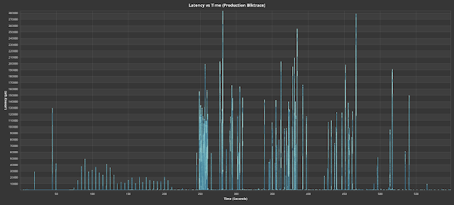
Fig. 5. Latency vs time for a production blktrace with a big
data workload
Since we control the “production” environment, we’ve taken
this same drive over to an Oakgate replay appliance and ran a replay file
generated from Fig. 4’s workload. We iterated multiple rounds of replay
(preconditioning between each iteration) and took those results and fed it back
into WI Analytics for comparison. Fig. 6 shows 3 iterations of the replay.
Fig. 6. Latency vs time for three rounds of replay
In a quick glance, we can see that the latency spikes and
their timings for the replayed results are extremely similar to the original
production trace. There are some statistical differences, if we closely, which
is expected. Overall, the replays have faithfully regenerated the latency
profile in an offline environment, and this particular drive has shown stable
results after multiple rounds of replay.
Replay Comparison for Different SSDs
Next, let’s run experiments on how different SSDs react to
the same workload. Such a use case can very well be used to qualify different
drives for a data center’s set of workloads. From a different angle, the same
experiment can be run on the same SSD with different firmware to see if
firmware changes are effective against a particular set of workloads.
In these experiments, we had chosen an actual data center
workload that showed a particularly stressful profile. Fig. 7 shows the read latency
vs. time of the production workload. We can see very big latency spikes happen,
and we would like to know whether other SSDs can handle this same workload
without these latency spikes. Fig. 8 shows the main obstacle the workload
entails – a burst of large discard (trim) IOs that is likely causing the disk
to become blocked while servicing those discards, contributing the high read
latency spikes.
Fig. 7. Data center production blktrace.
Fig. 8. Discard (trim) IO sizes vs time for production
blktrace.
Fig. 9 shows drives from various vendors that did not
encounter the read latency spikes despite undergoing the same production
workload. Latency scales are normalized to that of the production workload the
contrast the latency differences.
Fig. 9. Workload replayed against drives that did not show latency
spikes.
By contrast, Fig. 10 shows the set of drives that show an
adverse reaction to the burst of discard IOs. Vendor F in particular never
recovered to its baseline latencies after getting swamped with the discard
bursts.
Fig. 10. Drives that reacted adversely to the replayed
production workload.
Conclusion
The ability to replay production storage workloads is an
essential tool to improving or qualifying SSD real-world performance. Unlike
synthetic workloads, production workloads are much more unpredictable, dynamic,
and reflective of real application environments. In this blog, we discuss the
various aspects of accurately replaying workloads in an offline environment and
showed examples on how to properly reproduce production environments. We also
showed how different SSDs can react very differently to the same production
workload. Hopefully, we’ve conveyed the point that it is essential to use
real-world replays to design better SSDs and better match sets of SSDs relevant
to one’s real-world environment.
By Fred Tzeng, Ph.D. Software Architect
OakGate Product Family, Teledyne LeCroy
Learn more about Teledyne LeCroy
OakGate Products

 will \"impersonate\" the WaveRunner 9404 on which the file was saved.")


