A Real-World FFT Example

Figure 1: Shown at top right is the output of a
5V switch-mode power supply acquired
with an RP4030 active voltage-rail probe

Performing a fast Fourier transfer (FFT) on an oscilloscope can be likened to driving a car. Just as there are two dominant strains of power-train transmissions, there are two dominant approaches to transferring signals acquired on an oscilloscope from the time domain to the frequency domain. There's the stickshift approach, in which the FFT parameters are set manually, and the automatic approach, in which you let the oscilloscope make decisions for you.

Fast Fourier Transforms: Automatic Edition

Figure 1: Shown is the user interface for Teledyne LeCroy's
Spectrum Analyzer software option

Many motorists love the experience of driving a sporty car with its convertible top down and a stickshift manual transmission. Others don't want the hassle of a clutch and prefer the user-friendly feel of a slick automatic that does some of the work for them. Oscilloscopes can provide the same sort of choice for many measurement tasks in the same instrument.

Fast Fourier Transforms: Stickshift Edition

Figure 1: Shown at left is a 50-kHz input sine wave
with the FFT of the same signal at right

Perhaps you're old enough to remember when more cars had stickshifts. They're a little bit more work to drive than cars with automatic transmissions, but the experience can be much more rewarding. Oscilloscopes these days are like cars with both types of transmissions, and you can use either one for many tasks. One of those tasks is fast Fourier transforms (FFTs), and in this post we'll take you through driving an oscilloscope to perform an FFT with a stickshift.

Which Windowing Function to Use in FFTs?

Figure 1: Examples of a Hamming
function (blue) and Hanning function
(red)

When performing a fast Fourier transform on an acquired waveform, you'll often encounter situations where the waveform doesn't sit neatly within the oscilloscope's acquisition window so that the voltage is the same at the window's beginning and end. The ensuing discontinuity from window to window results in high-frequency artifacts, and the way to address this issue is a technique known as "windowing."

About Windowing in Fast Fourier Transforms

Figure 1: Windowing a waveform that's not periodic within
the acquisition window reduces spectral leakage

The second artifact in FFT calculations is more serious and is also the source of some confusion. A good source for information on this topic of windowing is an application note published by National Instruments.

About Data Truncation in Fast Fourier Transforms

Figure 1: The first precondition of using the Fourier transform
is a repetitive signal

Our last post discussed how time-domain signals acquired by an oscilloscope might be translated into the frequency domain using the discrete Fourier transform. We noted that using the Fourier transform only works if our signal is repetitive (Figure 1), and that it allows us to identify only harmonics of the first harmonic frequency, which is 1/acquisition window. Moreover, the discrete Fourier transform, if used on a large number of data points, is relatively slow to calculate.

Getting From the Time Domain to the Frequency Domain

Figure 1: A fundamental underlying assumption of a discrete
Fourier transform is a repetitive waveform

Fundamentally, oscilloscopes are time-domain instruments: We use them to acquire signals from our circuitry or device under test, and the instrument displays them in the time domain. We see the voltage of the signal in the vertical axis, and we see how that voltage changes over time in the horizontal axis.

Investigating IoT Wireless Signals (Part II)

Figure 1: This screen capture depicts frequency demodulation
and subsequent Manchester decoding of the bit stream

Internet of Things (IoT) devices must communicate with their peers--other IoT devices--as well as with the host system that governs their activities. In our previous post, we examined how to perform amplitude and frequency demodulation of RF bursts, such as Bluetooth Low Energy (BLE) advertising bursts. We'll continue with other methods of analyzing RF signals.

Getting The Most Out Of Your Oscilloscope: Math Functions

Figure 1: Parameter math functions
provide a way to create custom
parameters

Parameter math functions are an important part of an oscilloscope's analysis capabilities. Using parameter math, you can create custom parameters based on simple arithmetic relationships between existing parameters. It allows you to add, subtract, multiply, divide, or rescale parameters (Figure 1).

Probing Techniques and Tradeoffs (Part III)

Figure 1: Bandwidth is defined as the frequency at which
the ratio of the displayed amplitude to the input amplitude
is -3 dB (or 0.707)

Any discussion of oscilloscopes and/or probes must include the topic of analog bandwidth. Bandwidth is one of a short list of key specifications for a testbench setup. All oscilloscopes and probes come to market with a bandwidth specification, which is defined as:

The frequency at which the ratio of the displayed amplitude to the input amplitude is -3 dB (or 0.707).

This is known as the "-3 dB point," or the half-power point (Figure 1). At this frequency, a sine-wave input signal is attenuated to 70.7% of its true amplitude. Any higher frequencies will likely be distorted on the display, making accurate measurements and calibration impossible.

The Periodic Table of Oscilloscope Tools: Math

Figure 1: DSP-based
Math functions can
reveal deep insights
hidden in waveforms

The usefulness of oscilloscopes skyrocketed once digital signal processing began to be applied to acquired waveforms. By applying DSP, oscilloscopes could now perform complex processing in the time, frequency, statistical, and other domains, all while imposing no restrictions on acquisition length. Here at Teledyne LeCroy, we collectively refer to these DSP-based processes as Math functions. We've presented those functions, along with all of the other functions our instruments perform, in chart form in our Periodic Table of Oscilloscope Tools.

Follow The Bouncing Signal

Figure 1: Trend plotting is a handy tool
for discerning frequency-hopping
patterns

Signal jamming, noise generation/interference, signal interception, and other malicious RF-related activities have long been part and parcel of the electronic warfare arena. One countermeasure that is widely deployed is frequency hopping spread-spectrum (FHSS) transmission, or rapid and pseudo-random jumps of the carrier frequency in an effort to confound would-be jammers. FHSS transmission poses test and measurement challenges that we'll outline below.

The History of Jitter (Part V)

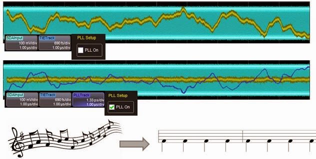Figure 1: Applying PLLs for clock-data recovery is not
unlike tapping your feet to the beat of music

A milestone in the history of jitter measurement came in the 1990s with receivers that could reveal the slowly varying component of jitter that became evident in time-interval error (TIE) tracks. That led to the advent of using phase-locked loops (PLLs) for clock-data recovery. In turn, PLLs opened new horizons in jitter analysis.

Going From FFTs to Spectrum Analysis

Figure 1: Spectrum Analyzer software for the HDO series
oscilloscopes provides an intuitive user interface

In earlier posts, we looked at a) the basics of fast-Fourier transforms (FFTs) and b) how to set up an FFT on a modern digital oscilloscope. In this post, we'll take a brief look at what that modern scope can do with an FFT, provided that scope is outfitted with software that will let it take full advantage. After all, the object of an FFT is to transform a time-domain waveform into the frequency domain. Sounds kind of like a spectrum analyzer, no?

Back to Basics: What is an FFT?

Figure 1: An FFT of a 300-kHz square wave.

In an earlier post, we discussed the basics of setting up a fast-Fourier transform (FFT) on an oscilloscope, and why you'd want to use an FFT to get a frequency-domain view of a time-domain signal in the first place. It might be a good idea to take a step back and dig into just what an FFT is (Figure 1).

Oscilloscope Basics: Setting Up FFTs

Figure 1: Capture time determines the
frequency resolution, Δf.

For most of their history, oscilloscopes have been thought of chiefly as a time-domain instrument. That is, an oscilloscope facilitates the observation of changes in a signal's amplitude over time. However, many modern digital and mixed-signal oscilloscopes provide spectral analysis capabilities based on fast Fourier transforms (FFTs) that convert a time-domain waveform into the frequency domain. There are lots of good reasons for taking advantage of this capability. Perhaps the most important is to gain insight into characteristics of the signal that simply are not apparent from a time-domain perspective.