You need to test, we're here to help.

You need to test, we're here to help.
Showing posts with label oscilloscope basics. Show all posts

13 June 2022

Oscilloscope Basics: Cal Out and Aux Out

Figure 5. New PCIe 6.0 compliance pattern signal.
Fig. 1: Cal Out and Aux Out 
provide many useful outputs.
Oscilloscopes are generally thought of in terms of the signals that are input to them, but even oscilloscopes that are not equipped with function/signal generators can usually output some useful test signals.

Nearly all oscilloscopes have a Cal Out (calibration output) terminal on the front. Most Teledyne LeCroy oscilloscopes also have an Aux Out (auxiliary output) connector on either the front or back, depending on  model. Both outputs provide configurable signals that can assist you to compensate probes and attenuators, test frequency response, trigger waveform acquisition and coordinate multiple test instruments.

16 May 2022

Oscilloscope Basics: External, Line and Fast Edge "Triggers"

An oscilloscope trigger synchronizes the oscilloscope timebase to the input signal so that the displayed trace is stable. In digital storage oscilloscopes, while the digitizer runs continuously converting analog voltage/current inputs to digital values, it is the trigger event that defines the “acquisition window,” marking the point where data is stored to acquisition memory, locking the signal data for display, measurement and further processing. 

Figure 1: The trigger setup showing the possible choices for the trigger source.

Triggers are set to fire based on the state of a trigger source waveform. What are commonly known as External, Line and Fast Edge "triggers" are not really different trigger types, per se, but alternative trigger sources.  Figure 1 shows the typical setup options for an Edge trigger, the most commonly used trigger type.  With Edge triggering, the oscilloscope is triggered when the source waveform crosses a user-defined threshold level and slope.  Usually, the source will be analog input channel C1-Cn. However, three other sources can be used to initiate an Edge trigger: an Ext(ernal) input, the Line (mains) power and, on some oscilloscopes, the built-in Fast Edge signal. 

04 April 2022

Oscilloscope Basics: When to Use Trend to Graph Oscilloscope Measurements

Figure 1: Applying the Trend operator to the same input waveform illustrates how the Trend is asynchronous to the input waveform.
Figure 1: Applying the Trend operator to the
same input waveform illustrates how the
Trend is asynchronous to the input waveform.  
In a previous post, we described the characteristics of the Track math function and two key applications of using Tracks to graph oscilloscope measurement data: anomaly detection and waveform demodulation. In this post, we'll discuss the characteristics and uses of the Trend function.

To illustrate an important distinction between Tracks and Trends, the Trend math operator in Figure 1 is now applied to the same signal as was the Track in our previous post without first reacquiring the input waveform. 

Note that unlike a Track, the Trend is not time-synchronized to the input waveform. Only the order of events, and not the timing of events, is retained. The underlying shape of the Track may be displayed in the Trend because the same measurement values from a single acquisition are displayed in the same sequence—however, the timing information of when each of the values has occurred is not retained in the Trend. Therefore, unlike the Track, the Trend does not point to the location of an anomaly. Without time scaling, the Trend does not have the frequency information needed to demodulate an input waveform.

28 March 2022

Oscilloscope Basics: When to Use Track to Graph Oscilloscope Measurements

Figure 4: The Trend (green) retains a history of pulse widths, while the Track (blue) shows only a flat line corresponding to the most recent width.
Figure 1: Pulse Width Modulated waveform (yellow)
and Track math operator (blue),
where the X-axis scaling is identical for both.
Modern oscilloscopes contain many tools that can be used for analyzing data, including Track and Trend math functions. Both Tracks and Trends graphically display measurement results and locate anomalies. The main similarity between Tracks and Trends is that the Y-axis of both operators is the measurement parameter itself (for example, Pulse Width, Duty Cycle, Rise Time, Slew Rate, etc.). The main difference between the two math operators is their X-axis, in which the Track uses the identical X-axis and synchronous horizontal scaling as the input waveform, whereas the Trend uses units of chronology. A Track, in essence, is a waveform of the measurement values. A Trend is a data logger showing the history of change in measured parameter values, but points are not necessarily synchronous with the measured waveform.

Use Tracks for Anomaly Detection

The Track provides valuable debugging information by directly pointing to an area of interest. 

Notice the negative-going spike in the Track waveform in Figure 1. Figure 1 occurs at the point in time where the input waveform reaches its most narrow pulse width, and the Track instantly finds it, indicating when one measurement deviates from the others in the graph. The Track identifies the exact location in time where the narrowest or widest pulse width has occurred, and fully describes the measurement changes occurring throughout the entire waveform. Since oscilloscopes can acquire thousands or even millions of waveform edges within a single acquisition, the Track allows an engineer to quickly "find the needle in a haystack".

10 January 2022

Oscilloscope Basics: Stabilizing Waveform Display, Pt. 2

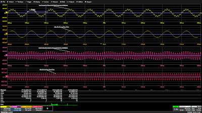
Figure 1: A 50 kHz low-pass filter eliminates a 93 kHz interfering signal from a 10 kHz signal (top two grids) and a 50 kHz high-pass filter cleans up a 93 kHz signal with an additive 10 kHz interfering signal (bottom two grids). Click image to expand.
Figure 1: A 50 kHz low-pass filter eliminates a
93 kHz interfering signal from a 10 kHz signal (top two grids)
and a 50 kHz high-pass filter cleans up a 93 kHz signal
with an additive 10 kHz interfering signal (bottom two grids).
Click image to expand.
In Pt. 1, we discussed the fundamental cause of unstable waveform displays. In this post, we’ll discuss how to use signal conditioners and conditional triggering to help the oscilloscope ignore extraneous samples when determining where the acquisition trigger event actually occurs.

Coupling 

In the Setup section of the Trigger dialog, Trigger input sources can be conditioned using AC or DC coupling, high-pass filters (LFREJ for low-frequency reject) and low-pass filters (HFREJ for high-frequency reject). The frequency selective coupling paths are used to attenuate extraneous signals. The low-frequency reject inserts a 50 kHz high-pass filter in the trigger signal path, which is useful for eliminating low-frequency interference such as 60 Hz power mains signals. This low-frequency noise can cause erroneous triggers, resulting in an unstable display. The high-frequency reject inserts a 50 kHz low-pass filter. This coupling mode finds use in applications such as troubleshooting switch-mode power supplies, where it suppresses signals at the power supply switching frequency. Like any extraneous signal, high frequency pickup can leak into the input signal and cause trigger instability. Figure 1 provides examples of how the HFREJ and LFREJ coupling filters eliminate interfering signals from the trigger source.

04 January 2022

Oscilloscope Basics: Stabilizing Waveform Display, Pt. 1

Figure 1: A free running oscilloscope starts each acquisition at a different point on the waveform, resulting in an unstable display.  A triggered oscilloscope starts each acquisition at the same point on the waveform, resulting in a stable display.
Figure 1: A free running oscilloscope starts each
acquisition at a different point on the waveform,
resulting in an unstable display.  A triggered oscilloscope
starts each acquisition at the same point on the
waveform, resulting in a stable display. 
An unsynchronized, unstable oscilloscope display is useless for making measurements, but proper triggering can synchronize the oscilloscope sample clock to specific waveform events so that the acquired waveforms appear stable on the display.  Let’s look at why signals can appear unstable and what to do about it.  

Oscilloscopes are sampling devices; they sample the incoming signal at a uniform rate.  The timing of a signal applied to the input of an oscilloscope is most probably asynchronous with the oscilloscope’s sampling clock.  If the oscilloscope timebase is allowed to run free—that is, not synchronized to the timing of the input signal—then each oscilloscope acquisition potentially begins at a different point on the input waveform, as shown in Figure 1.

30 November 2020

Oscilloscope Basics: Multiplexed Front Panel Controls

Fig. 1. Modern, slim front panel.
Fig. 1. Modern,
slim front panel.
Most Teledyne LeCroy oscilloscopes are equipped with traditional front panel controls—knobs and buttons—that are a (literally) handy way to make basic acquisition settings such as gain, timebase and trigger level. While all these could be made using the oscilloscope software, using the front panel allows you to keep dialogs closed and more of the screen “real estate” available for viewing traces as you modify these settings.

In order to optimize that real estate, front panels have become increasingly slim, and many front panel controls on newer Teledyne  LeCroy oscilloscopes are multiplexed, meaning they have multiple functions or can be used to control multiple on-screen objects. Here is a list of tips to keep in mind when using the front panel.

27 March 2015

Oscilloscope Basics: Choosing an Oscilloscope

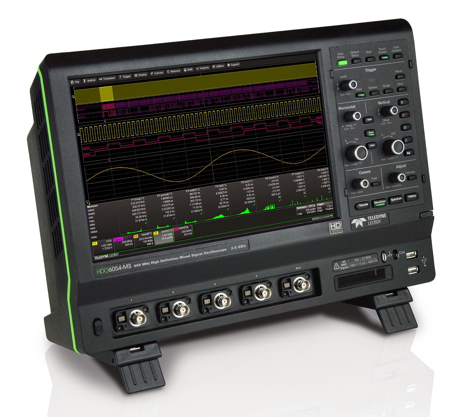
An oscilloscope such as Teledyne LeCroy's HDO6054-MS serves a very broad range of applications
Figure 1: An oscilloscope such as
Teledyne LeCroy's HDO6054-MS
serves a very broad range of
applications
Choosing an oscilloscope might seem to be a challenging task, but it doesn't have to be. Rather, it's a more-or-less logical process based on your measurement needs. Having said that, if the application for the instrument is "general lab work," the decision can become trickier.

05 September 2014

Oscilloscope Basics: Using The Display Graticule

The oscilloscope display graticule
Figure 1: The display graticule, the grid of intersecting lines
overlaying the signal display area, is the original
oscilloscope measurement tool
Today's digital oscilloscopes come packed with an abundance of measurement capabilities, all available at the touch of a button or two. Want to know the amplitude of a square wave? Easy. Want to know the standard deviation of that amplitude? Minimum/maximum or mean? All easily compiled for you over hundreds or thousands of acquisitions.

05 August 2014

Oscilloscope Basics: History Mode

Initial setup of WaveSurfer 3000 oscilloscope
Figure 1: Initial setup of WaveSurfer 3000 with a
2-MHz pulse waveform fed into Channel 1
Back in the day, one of the biggest deficiencies of early digital oscilloscopes was their lack of memory depth. A memory of 500 or 1000 points was about as good as it got, and this didn't provide much in the way of detailed waveform capture. Today's instruments are very different animals; for example, Teledyne LeCroy's recently introduced WaveSurfer 3000 oscilloscopes offer up to 10 Mpoints of memory per channel.

18 December 2013

Oscilloscope Basics: Trigger Holdoff

As discussed in an earlier post, triggering is the means by which we can coax an oscilloscope into showing us what we're looking for in an input signal, and indeed even simply to display it in a stable fashion. Two of the most basic triggering types are edge triggers and pattern triggers. The latter applies to mixed-signal instruments, allowing users to trigger on a logical combination of analog and digital inputs.

30 October 2013

Oscilloscope Basics: Controlling an Oscilloscope (Part II)

An example of a touch screen-equipped oscilloscope.
Figure 1: An example of a
touch screen-equipped
oscilloscope.
In a recent post, we discussed how to control a modern digital oscilloscope using the front-panel controls. That was a natural place to begin, given that it's the "traditional" means of controlling the instrument and the one that most seasoned users cut their teeth on. But there's more than one way to skin this cat these days. Many of today's oscilloscopes carry touch screens that do everything the front-panel controls can do, plus some things they cannot do.

23 October 2013

Oscilloscope Basics: How to Set Up and Use Cursors

As a follow-up to a recent post with an oscilloscope front-panel tour, we want to dig a little deeper into one aspect of controlling the instrument, and that's how to set up and use cursors. But instead of describing it in prose, it makes more sense to show you. So enjoy this brief tutorial video that will get you started with cursors! We're demonstrating on a Teledyne LeCroy HDO4054, but most of what we're showing you translates to other manufacturer's instruments.

02 October 2013

Oscilloscope Basics: Controlling An Oscilloscope (Part I)

Front of HDO6054 oscilloscope
Figure 1: Front of HDO4054 oscilloscope
At first glance, the front of today's oscilloscopes can be daunting. For starters, there's an array of physical "hard" controls. Relatively recent models may also sport touch screen displays with so-called "soft" controls. For one thing, getting familiar with the front of these instruments is only a matter of experimentation and common sense. And for another, what at first may seem complex is carefully designed to make the instrument as easy to operate as possible. This is the first installment of a projected series of posts that will explain how to control a modern oscilloscope. Here, we'll start with the front panel.

30 August 2013

Oscilloscope Basics: Setting Up FFTs

Capture time determines the frequency resolution, Δf
Figure 1: Capture time determines the
frequency resolution, Δf.
For most of their history, oscilloscopes have been thought of chiefly as a time-domain instrument. That is, an oscilloscope facilitates the observation of changes in a signal's amplitude over time. However, many modern digital and mixed-signal oscilloscopes provide spectral analysis capabilities based on fast Fourier transforms (FFTs) that convert a time-domain waveform into the frequency domain. There are lots of good reasons for taking advantage of this capability. Perhaps the most important is to gain insight into characteristics of the signal that simply are not apparent from a time-domain perspective.

10 June 2013

Oscilloscope Basics: Sampling Rate

In a recent overview post on oscilloscope banner specifications,
one of the topics covered is sampling rate. Let's do a somewhat deeper dive on that topic and look at what sampling rate means to oscilloscope users.

17 May 2013

Oscilloscope Basics: Triggering

At some point, it's likely you've had the experience of capturing a waveform on your oscilloscope only to see a wildly unstable trace displayed on the screen. Chances are that you hadn't adjusted the triggering correctly. Let's take a brief look at what triggering is and why it's important in an oscilloscope. Trigger modes determine when the oscilloscope acquires and what is displayed.

01 April 2013

Oscilloscope Basics: Oscilloscope Bandwidth

Among the most important basic specifications of a digital oscilloscope is its bandwidth. Knowing a bit about bandwidth and the influences on the specification can be very helpful in selecting the right oscilloscope for your application. This post will cover some fundamental aspects of oscilloscope bandwidth.