Back to Basics: Three-Phase Sinusoidal Voltages

Figure 1: Three-phase AC voltages
consist of three voltage vectors

In a previous post, we briefly covered the basics of single- and three-phase AC power systems. Single-phase systems, as we've noted, comprise a single voltage vector with a magnitude (in VAC) and a phase angle. Of course, a three-phase voltage consists of three voltage vectors and three phase angles. This installment will go on to describe three-phase AC voltages in similarly brief fashion.

Back to Basics: Fundamentals of AC Line Power (Part II)

Figure 1: AC line voltage is a single-phase
vector that rotates at a given frequency

Having reviewed a broad definition of power, how it is generated and distributed, and how motors consume almost half of all generated power, we will now turn to a more detailed discussion of just what it is that we call "power." When we discuss "power," we're typically referring to what comes out of a wall socket: AC line, or sinusoidal, power.

Oscilloscope Basics: History Mode

Figure 1: Initial setup of WaveSurfer 3000 with a
2-MHz pulse waveform fed into Channel 1

Back in the day, one of the biggest deficiencies of early digital oscilloscopes was their lack of memory depth. A memory of 500 or 1000 points was about as good as it got, and this didn't provide much in the way of detailed waveform capture. Today's instruments are very different animals; for example, Teledyne LeCroy's recently introduced WaveSurfer 3000 oscilloscopes offer up to 10 Mpoints of memory per channel.

Back to Basics: S-parameters

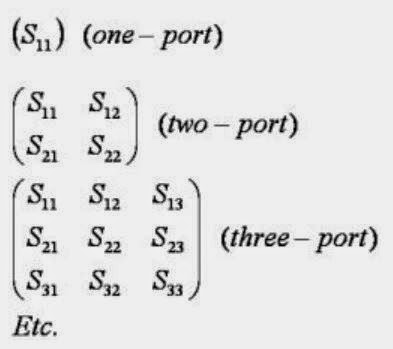Figure 1: S-matrices for one-, two-,
and three-port RF networks

Suppose you have an optical lens of some sort onto which you shine a light with a known photonic output. While most of the incident light passes through the lens, some fraction of the light is reflected and some is absorbed (the behavior is also dependent on the wavelength of the incident light). You'd like to characterize that lens: Exactly how much light was reflected? How much passed through? What is it about the lens that prevented all of the light from passing through?

Back to Basics: Jitter

Figure 1: Jitter is short-term variation
of a signal with respect to its
ideal position in time

Anyone working in applications that involve digital data, clocks, and serial data in general will eventually bump up against issues concerning jitter. Jitter is a subject of keen interest to every strata of the electronics industry. Chip makers, board integrators, system integrators, you name it: Everybody wants, and needs, to come to terms with jitter. It impacts reliability, manufacturability, and cost at all levels. And, of course, it's of keen interest to purveyors of test instruments, including us here at Teledyne LeCroy. In this first post of a projected series on jitter, we'll look at some of the tools built into modern digital oscilloscopes for jitter measurement and analysis.

Oscilloscope Basics: Trigger Holdoff

As discussed in an earlier post, triggering is the means by which we can coax an oscilloscope into showing us what we're looking for in an input signal, and indeed even simply to display it in a stable fashion. Two of the most basic triggering types are edge triggers and pattern triggers. The latter applies to mixed-signal instruments, allowing users to trigger on a logical combination of analog and digital inputs.

Back to Basics: Probes (Part IV)

Figure 1: An example of
differential probes
measuring from test
point to test point.

In three earlier posts on the basics of oscilloscope probes, we've taken a broad overview approach, looked more deeply at passive probes and inductance effects, and most recently, dug into active probes. Next up is differential probes, a different animal entirely from the foregoing types.

Back to Basics: Probes (Part III)

Figure 1: Active oscilloscope probes
sport high resistance and low
capacitance at their tips, but
terminate into a scope's 50Ω input.

In the first two installments of this series on probe basics, we examined some broad probe categories (Part I) and some of the issues that come with probe inductance (Part II). In the present installment, we'll delve a bit deeper into the topic of active probes. We'll also discuss when it's best to use passive probes and when to use active types.

Back to Basics: Probes (Part II)

In a previous post, we provided some basic information about oscilloscope probes, including a brief survey of the different types and what can happen when the probe is connected to a DUT. In this installment, let's continue along those lines and take a closer look at passive probes.

Back to Basics: Probes (Part I)

Figure 1: An example of an active

oscilloscope probe 

To speak of an oscilloscope probe is to open a fairly large can of worms. There are many kinds of probes on the market, with differing functions and characteristics (Figure 1). This is the first in a short series of posts on the basics on probes, what the various kinds are used for, and how they might be expected to affect measurements taken with them.

Back to Basics: What is an FFT?

Figure 1: An FFT of a 300-kHz square wave.

In an earlier post, we discussed the basics of setting up a fast-Fourier transform (FFT) on an oscilloscope, and why you'd want to use an FFT to get a frequency-domain view of a time-domain signal in the first place. It might be a good idea to take a step back and dig into just what an FFT is (Figure 1).

Back to Basics: Creating Pulsed Waveforms

Figure 1: The Pulse
waveform dialog box.

Many test applications call for the creation of pulsed waveforms ranging from clock signals to logic control to trigger signals, among others. Often, these waveforms are used in the characterization and debug of digital devices and circuits. Stand-alone pulse generators provide one way to generate pulsed waveforms but in many cases, a general-purpose waveform generator will do a fine job.

Back to Basics: Differential Probing

Figure 1: Emitter voltage measurement
in simplified schematic view

Whether or not we think of it in such terms, any voltage measurement taken with an oscilloscope or voltmeter is, in reality, a differential voltage measurement. A voltage is, by definition, the difference in electrical potential between two points in a circuit. It's impossible to take a voltage measurement with only one voltmeter lead. One lead must be attached to the point of interest while the other must be connected somewhere else as a reference point.

Back to Basics: Sequence Mode

Figure 1: Sequence mode enables fast trigger rates
and optimizes memory usage by
ignoring dead time.

Now and again, an oscilloscope user may need to capture either a large number of fast pulses in quick succession, or a small number of events separated by relatively long periods of time. Either of these scenarios are challenging with typical acquisition modes. Fortunately, most modern oscilloscopes offer what we call "sequence mode" (other oscilloscope makers refer to similar acquisition modes as "fast-frame" or "segmented memory" mode).

Back to Basics: Random Interleaved Sampling

Figure 1: This image illustrates the
general principle underlying RIS.

Modern oscilloscopes come with all kinds of bells and whistles, and users might be tempted to invoke them for all sorts of situations. But not every whiz-bang feature of an oscilloscope is applicable all the time. Rather, some features are great in the right applications but disastrous in others.

Oscilloscope Basics: Triggering

At some point, it's likely you've had the experience of capturing a waveform on your oscilloscope only to see a wildly unstable trace displayed on the screen. Chances are that you hadn't adjusted the triggering correctly. Let's take a brief look at what triggering is and why it's important in an oscilloscope. Trigger modes determine when the oscilloscope acquires and what is displayed.

Oscilloscope Basics: Oscilloscope Bandwidth

Among the most important basic specifications of a digital oscilloscope is its bandwidth. Knowing a bit about bandwidth and the influences on the specification can be very helpful in selecting the right oscilloscope for your application. This post will cover some fundamental aspects of oscilloscope bandwidth.