You need to test, we're here to help.

You need to test, we're here to help.
Showing posts with label histogram. Show all posts

28 February 2022

Signal and Power Integrity Tutorial: A Robust Method for Measuring Clock Jitter with Oscilloscopes

Figure 1. Clock jitter measured as a variation of clock signal absolute period.
Figure 1. Clock jitter measured as a variation
of clock signal absolute period.
Clock jitter is the variation of a clock signal’s frequency or period. Either measurement carries the same information, but the period measurement is a simple time interval measurement easily performed using a real-time oscilloscope. If we have a robust way of measuring clock jitter, we have the basis for measuring the clock signal’s sensitivity to other features in the environment that can affect the period. Voltage noise on the power rail is just one external force that can affect clock jitter, which we'll show you how to measure in a future post.

In this post, we’ll demonstrate a robust method for measuring clock jitter using an example from Dr. Eric Bogatin’s webinar, “The Impact of Power Rail Noise on Clock Jitter.”  

The clock in our examples is a 5-stage ring oscillator which generates a square wave signal between 10 and 66 MHz. The test instrument is a WavePro HD 12-bit, 4-Ch, 8 GHz, 20 GS/s, 5 Gpts oscilloscope with 60 fs sample clock jitter.

In the process, we make a series of oscilloscope sample clock tests and timebase adjustments as  consistency checks. While measuring jitter is less about absolute accuracy than about the relative precision of measuring the time interval from cycle to cycle, a fundamental part of that is ensuring the absolute accuracy of the oscilloscope’s timebase.

25 October 2021

Measuring Dead Time in 48 V Power Converters, Part 2: Dynamic Measurements

Figure 1. P1 and P2 measure dt@lvl over the entire acquisition, while P3 and P4 measure dt@lvl for only a single operational cycle of zoom traces Z1 and Z3.
Figure 1. P1 and P2 measure dt@lvl over the entire acquisition,
while P3 and P4 measure dt@lvl for only a single operational
cycle of zoom traces Z1 and Z3.
A primary engineering task for 48 Volt power conversion systems using bridge topologies is to ensure adequate dead time to prevent catastrophic shoot through occurring when both HI and LO FETs conduct at the same time. Being able to accurately measure dead time is therefore of critical importance. Part 1 of this series dealt with the basic dead time measurement. Part 2 will deal with studying the dynamic changes in the dead time measurement using statistical tools like tracks and histogram functions. 

As we learned in part 1, the dead time delay is measured using two instances of the measurement parameter Delta Time at Level (dt@lvl) as shown in Figure 1. 

In the Figure 1, the dt@lvl parameters P1 and P2 show the value of the last measurement in the acquisition which contains 10,000 switching transitions. The parameters P2 and P4 measure only the single timing cycle shown in the zoom traces. (Click any  image to enlarge it and see the detail.)

The values of both parameters are different, and you should ask the question: how does dt@lvl vary with time? To find the answer, turn on the measurement parameter statistics, as shown in Figure 2.

12 April 2021

How to Use Measurement Statistics to Set Up Triggers

Figure 1.  Histogram of the different pulse widths occurring in a pulse-width modulated rectangular pulse train.
Figure 1.  Histogram of the different pulse widths occurring
in a pulse-width modulated rectangular pulse train.
Triggering is an essential element in all modern digital oscilloscopes.  The trigger synchronizes the oscilloscope’s data acquisition with a user-specified event on the signal, be that an edge, threshold crossing or a specific signal characteristic. Teledyne LeCroy Smart Triggers can trigger oscilloscope acquisitions based on properties such as a period, width, low signal amplitude, slew rate or signal loss. These trigger types are ideal for capturing transient events like glitches, but they require knowing at least a range of possible values for the trigger to detect.

Intermittent transient events and glitches are among the most frustrating problems to detect and solve. This is especially true if you have no idea about the nature of the transient. However, you can use the oscilloscope’s measurement tools to help locate these bothersome transients, then use that information to set up your trigger to capture them when they occur. Here’s how.

29 March 2021

How to "Layer" Measurement Tools

Figure 1: Multi-grid display "layers" multiple measurement tools to find hidden glitch.
Figure 1: Multi-grid display "layers" multiple
measurement tools to find hidden glitch.
Teledyne LeCroy oscilloscopes have four, distinct sets of measurement tools, including measurement graticules, cursors, parameters and graphs. These tools developed historically and are designed to be “layered” on multi-grid MAUI® oscilloscopes so that each addition brings a new level of understanding and insight. Even on oscilloscopes that do not have multi-grid displays, as shown here, several measurement tools can be applied at once for added insight. Read on to see how, properly combined, they can help you find waveform anomalies and assess their frequency of occurrence in a few, simple steps.

04 May 2018

Debugging Low-Speed Serial Data on IoT Devices

Serial-data links handle traffic between ICs and peripheral devices in the IoT world
Figure 1: Serial-data links handle traffic between ICs
and peripheral devices in the IoT world
Our last post discussed the difficulties in acquiring the many sensor signals that may be input to a deeply embedded system such as an IoT device as well as a hardware solution to the problem. Another aspect of IoT debugging and validation is the low-speed serial data standards used to facilitate communication between ICs and between controllers and peripheral devices (Figure 1). To that end, let's take a look at three such low-speed standards: I2C, SPI, and UART.

31 January 2018

Getting The Most Out Of Your Oscilloscope: Tracks and Trends

The track math function shows how data changes over time
Figure 1: The track math function
shows how data changes over time
Our discussion of cursors and parameters leads us neatly into the topics of tracks and trends, which are both means of extending parameter measurement into a more analytical direction. We can do this using math functions that are part of your Teledyne LeCroy oscilloscope's toolset.

30 January 2018

Getting The Most Out Of Your Oscilloscope: Cursors and Parameters

Cursors (top) and parameter measurements (bottom) are both powerful tools in their own right
Figure 1: Cursors (top) and parameter
measurements (bottom) are both
powerful tools in their own right
Oscilloscopes give us a wealth of tools with which to view, measure, and analyze the performance of a circuit. Broadly speaking, two classes of such tools are cursors and parameter measurements. Taken on their own, both classes afford the user a great deal of capability. Put them together, though, and you can really start to gain deep insights into what's going on with a waveform.

12 July 2017

The Periodic Table of Oscilloscope Tools: Measure

Measure tools are at the heart of an oscilloscope's utility
Figure 1: Measure
tools are at the heart
of an oscilloscope's
utility
An oscilloscope is only as good as the tools it provides to users for acquiring, viewing, measuring, analyzing, and documenting waveforms. We present an overview of our deep collection of oscilloscope tools in our Periodic Table of Oscilloscope Tools, and in prior Test Happens posts, we've surveyed the Capture and View categories. Today we'll break down the Measure section of the Table.

07 July 2017

The Periodic Table of Oscilloscope Tools: View

The View tools arrange acquisition data to suit given needs
Figure 1: The View tools
arrange acquisition data
to suit given needs
We began our survey of Teledyne LeCroy's Periodic Table of Oscilloscope Tools by reviewing our set of Capture tools, which help to isolate and capture signals of interest and shorten time to insight. Now we'll turn our attention to the next grouping of tools: the View tools.

30 November 2015

Follow The Bouncing Signal

Trend plotting is a handy tool for discerning frequency-hopping patterns
Figure 1: Trend plotting is a handy tool
for discerning frequency-hopping
patterns
Signal jamming, noise generation/interference, signal interception, and other malicious RF-related activities have long been part and parcel of the electronic warfare arena. One countermeasure that is widely deployed is frequency hopping spread-spectrum (FHSS) transmission, or rapid and pseudo-random jumps of the carrier frequency in an effort to confound would-be jammers. FHSS transmission poses test and measurement challenges that we'll outline below.

21 October 2015

Analyzing Pulse-Width Modulation Signals

Persistence display provides a quick-and-dirty view of a PWM signal
Figure 1: Persistence display provides
a quick-and-dirty view of a PWM signal
Pulse-width modulation (PWM), a favorite technique for achieving analog ends through digital means, finds application in all kinds of end systems. Motor control might be the number-one application, but PWM turns up in telecommunications, audio systems and amplifiers, and any number of other uses. Armed with a capable oscilloscope, one can thoroughly analyze and understand the behavior of PWM circuits.

01 October 2015

Taking Best Advantage of Oscilloscopes' Long Memory

Figure 1: Maintaining the maximum sample rate over more timebase settings is possible with long memory
Figure 1: Maintaining the maximum sample rate over more
timebase settings is possible with long memory
Two very important considerations when choosing a digital oscilloscope are the length of the acquisition memory and the amount of RAM available for processing of the raw data. Note that acquisition memory and RAM are not the same things, but they are still both important. The amount of acquisition memory often determines the fidelity with which an oscilloscope can record a signal. But that's only the first step; it's the instrument's processing horsepower is the key to finding signal abnormalities and characterizing circuit performance.

07 May 2015

Using Histograms (Part IV)

Figure 1: A histogram of delay between traces C1 and C2 with an unknown event occuring 2.5 ns outside of expected range
Figure 1: A histogram of delay between traces C1 and C2
with an unknown event occuring 2.5 ns outside of
expected range
In previous posts on the topic of histograms, we've considered examples of how looking at signals in the statistical domain in addition to the time and frequency domains can be a great aid in pinning down the root cause of problems. But what about going in the other direction? Suppose you spot something unusual in a histogram and want to examine the waveform?

02 April 2015

The History of Jitter (Part III)

Latching a signal at the outermost of the blue hash marks results in a BER of 10-3, while latching it at the innermost hash marks yields a BER of 10-12
Figure 1: Latching a signal at the outermost of the blue
hash marks results in a BER of 10-3, while latching it
at the innermost hash marks yields a BER of 10-12
If you've been keeping track of our history of jitter, we left off in Part II in the late 1990s, by which time bit-error rates (BER) had become a predominant statistic for quantifying jitter. That was subsequently refined into thinking in terms of BER as a function of jitter.

20 March 2015

Using Histograms (Part III)

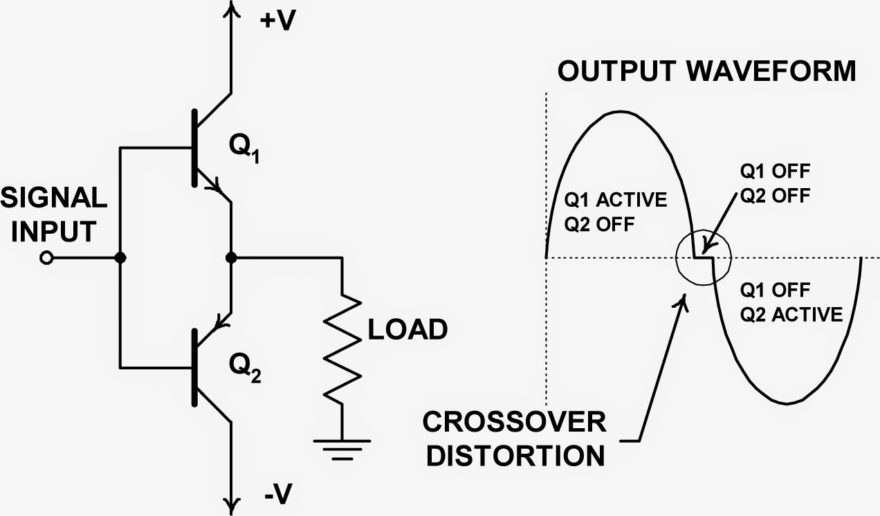
A simplified view of a push-pull amplifier showing the source of crossover distortion
Figure 1: A simplified view of a push-pull amplifier
showing the source of crossover distortion
In this third post in a series on using an oscilloscope's histogram capabilities, let's take a look at using histograms as a diagnostic tool. Diagnosing problems in a circuit calls for good skills and some intuition on top of good measurement tool. In general, though, the more ways in which you're able to look at a problem, the more likely it is that you'll turn up the root cause.

27 February 2015

Using Histograms (Part II)

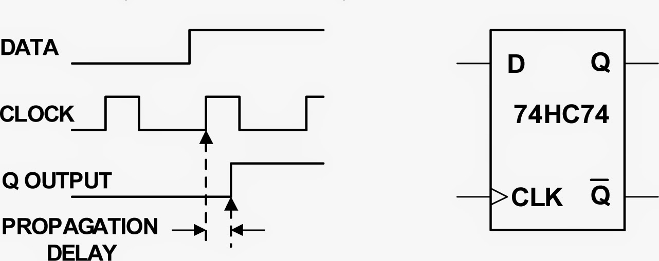
Figure 1: A flip-flop's propagation delay is a typical spec that can be derived using statistical analysis
Figure 1: A flip-flop's propagation delay is a typical spec
that can be derived using statistical analysis
In Part I of this series, we looked at some of the basics of histograms and how they can provide a statistical view into random variation of signal parameters. Next, let's look at how histograms can help us use statistical analysis to determine product specifications.

09 February 2015

Using Histograms (Part I)

Figure 1: Histograms of the period, width, and TIE show different distributions of time jitter
Figure 1: Histograms of the period, width, and
TIE show different distributions of time jitter
When we measure parameters of a waveform in a circuit or device, we rarely take a single measurement but rather a significant number of measurements. We want to see trends over time in the period, width, and time-interval error of a clock pulse, for example. Those parameters will have some nominal value, but there will typically be some random variation that we refer to as jitter.