Six Principles of FFT Analysis Using Real-time Oscilloscopes

Figure 1. A 100 MHz sine wave in the time domain
and its spectrum in the frequency domain showing
the one peak at 100 MHz. Click on any image to enlarge.

By Prof. Eric Bogatin,
Teledyne LeCroy Fellow

The following piece was published in Signal Integrity Journal and is excerpted here by permission of Signal Integrity Journal.

***************************

We live in the time domain. This is where we measure all digital performance. But sometimes, we can get to an answer faster by taking a detour through the frequency domain. With these six principles, we can understand how an oscilloscope transforms time domain measurements into a frequency domain view. All six principles are applied “under the hood” by oscilloscopes with a built-in FFT function. (Our note: Also by software packages designed for spectral analysis, such as the SPECTRUM-1 and SPECTRUM-PRO-2R options.)

1. The spectrum is a combination of sine wave components

In the frequency domain, the only waveforms we are allowed to consider are sine waves. There are other special waveforms combinations of which can describe any time-domain waveform, such as Legendre polynomials, Hermite polynomials or even wavelets. The reason we single out sine waves for a frequency domain description, is that sine waves are solutions to second order, linear, differential equations—the equations found so often in electrical circuits involving resistor, capacitor and inductor elements. This means signals that arise or have interacted with RLC circuits are described more simply when using combinations of sine waves than any other function because sine waves naturally occur. 

Oscilloscope Basics: Stabilizing Waveform Display, Pt. 2

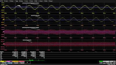
Figure 1: A 50 kHz low-pass filter eliminates a
93 kHz interfering signal from a 10 kHz signal (top two grids)
and a 50 kHz high-pass filter cleans up a 93 kHz signal
with an additive 10 kHz interfering signal (bottom two grids).
Click image to expand.

In Pt. 1, we discussed the fundamental cause of unstable waveform displays. In this post, we’ll discuss how to use signal conditioners and conditional triggering to help the oscilloscope ignore extraneous samples when determining where the acquisition trigger event actually occurs.

Coupling 

In the Setup section of the Trigger dialog, Trigger input sources can be conditioned using AC or DC coupling, high-pass filters (LFREJ for low-frequency reject) and low-pass filters (HFREJ for high-frequency reject). The frequency selective coupling paths are used to attenuate extraneous signals. The low-frequency reject inserts a 50 kHz high-pass filter in the trigger signal path, which is useful for eliminating low-frequency interference such as 60 Hz power mains signals. This low-frequency noise can cause erroneous triggers, resulting in an unstable display. The high-frequency reject inserts a 50 kHz low-pass filter. This coupling mode finds use in applications such as troubleshooting switch-mode power supplies, where it suppresses signals at the power supply switching frequency. Like any extraneous signal, high frequency pickup can leak into the input signal and cause trigger instability. Figure 1 provides examples of how the HFREJ and LFREJ coupling filters eliminate interfering signals from the trigger source.