Oscilloscope Basics: Stabilizing Waveform Display, Pt. 2

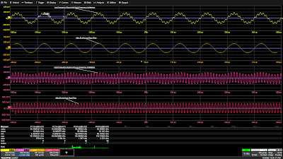
Figure 1: A 50 kHz low-pass filter eliminates a
93 kHz interfering signal from a 10 kHz signal (top two grids)
and a 50 kHz high-pass filter cleans up a 93 kHz signal
with an additive 10 kHz interfering signal (bottom two grids).
Click image to expand.

In Pt. 1, we discussed the fundamental cause of unstable waveform displays. In this post, we’ll discuss how to use signal conditioners and conditional triggering to help the oscilloscope ignore extraneous samples when determining where the acquisition trigger event actually occurs.

Coupling 

In the Setup section of the Trigger dialog, Trigger input sources can be conditioned using AC or DC coupling, high-pass filters (LFREJ for low-frequency reject) and low-pass filters (HFREJ for high-frequency reject). The frequency selective coupling paths are used to attenuate extraneous signals. The low-frequency reject inserts a 50 kHz high-pass filter in the trigger signal path, which is useful for eliminating low-frequency interference such as 60 Hz power mains signals. This low-frequency noise can cause erroneous triggers, resulting in an unstable display. The high-frequency reject inserts a 50 kHz low-pass filter. This coupling mode finds use in applications such as troubleshooting switch-mode power supplies, where it suppresses signals at the power supply switching frequency. Like any extraneous signal, high frequency pickup can leak into the input signal and cause trigger instability. Figure 1 provides examples of how the HFREJ and LFREJ coupling filters eliminate interfering signals from the trigger source.

How to Test Noisy Power Supply Outputs

Figure 1: 3.3 V output of a DC-DC converter.
The waveform shows the nominal DC level,
ripple and high frequency noise bursts.

Did you ever acquire the output of a power supply with your oscilloscope and find an unexpectedly high level of noise? Did you try adding filter capacitors only to find the noise level was not changed? 

In this post, we'll discuss how the choice of probe affects the noise present in power measurements, as well as how oscilloscope settings such as termination impedance, bandwidth and coupling can be adjusted to lessen noise and improve measurement results.

Figure 1 shows a typical DC-DC converter output measurement. The mean value of the waveform is 3.294 V.  Ripple appears at the switching frequency of 1.2 MHz, and noise in the form of high frequency bursts and baseline thickening is visible throughout.

Waveforms like this can be acquired with a 10:1 high impedance probe, a 1:1 coaxial cable connection, or a 1.2:1 rail probe using either DC or AC coupling, as available.  Figure 2 summarizes how each oscilloscope/probe configuration affects the measurement.

Fundamentals of Power Integrity: Board Pollution

Figure 1. "Pollution" occurring on PDN traces.

Board pollution is noise occurring on the packages and interconnects (traces and planes) that carry current from the VRMs to the consumer devices.
One place it can originate is from the VRM itself, for example, with the switching noise the VRM generates (Figure 1). That can be a real concern if the board capacitance means you have a resonance around the switching frequency that would act as an amplifier for the switching noise and cause all kinds of problems with other devices on the board.

Fundamentals of Power Integrity: Self-aggression Noise

Fig. 1: VRM-switching noise is a self aggressor that can be
identified because it is synchronous with the PWM clock. 

Self-aggression noise is so-called because it is inflicted by a component onto itself through its normal operation; nothing else in the system is affecting it. When we look for this, we want to ensure the system is in a steady state, in a place where the noise environment is fairly clear (e.g., the device is on an evaluation board).

An example of self-aggression would be VRM-switching noise. Figure 1 shows ripple on a 900 millivolt rail (yellow trace) at a time when no load is present. One of the things that tells us this is switching noise is that it is synchronous to the PWM clock (red trace). Ripple that is synchronous with the switching clock is a typical figure of merit for identifying switching noise.

Fundamentals of Power Integrity: Characterizing PDN Noise

Figure 1. Noise tolerances for embedded system
components are becoming ever tighter.

Power integrity concerns maintaining the quality of power from generation to consumption in an embedded system. “Good” power integrity could be defined as having noise levels that are within tolerance. This short series will focus on characterizing noise on your power delivery network (PDN), with the goal of knowing where you must adjust your design to meet those tolerances.

Why do we care about voltage rail noise? As electronic designs strive for ever lower power consumption, power rails already carry very low voltages, often 1 V or less. Components like RF receivers, ADCs and DACs can be affected by noise of less than 1% of the rail value (Figure 1). This means noise tolerances can be as tight as single-digit millivolts, which is why power integrity takes up considerable validation time in labs.

Just the FAQs: Waveform Averaging

Figure 1: The upper grid displays raw samples directly from
the ADC; the lower grid displays the average of 1000
acquisitions.

If you've poked around the Teledyne LeCroy website, perhaps you've run across the extensive (and growing) collection of test-related tidbits we call our FAQ Knowledgebase. To highlight some of these helpful hints for making better use of your oscilloscopes, protocol analyzers, network analyzers, etc., we'll post some here on the Test Happens blog from time to time.