 |
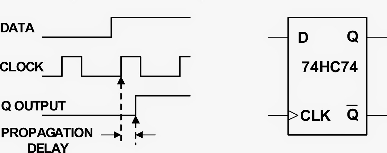
Figure 1: A flip-flop's propagation delay is a typical spec
that can be derived using statistical analysis
|
Many of Teledyne LeCroy's oscilloscopes are able to create statistical-analysis histograms on a very large number of measurements. The resulting data can be displayed as histograms, as trend plots (measurements in the order taken), or as track plots (measurements vs. time). As a result, the analysis capabilities of these instruments is extended to cover accurate readouts of up to 20 key statistical measurements such as mean, standard deviation, range, and many more.
 |
Figure 2: At right is a histogram showing the distribution of
over 46,000 measurements of the propagation delay of a
74HC74 D-type flip flop at 25°C
|
In Figure 2, the upper left-hand trace (Ch1) is the clock. Below that is the Q output (Ch2), while the right-hand trace (M1) is the histogram of the delay between positive-going edges of the clock and the Q output. The histogram shows the distribution of over 46,000 individual measurements. Meanwhile, the statistical parameters, histogram mean, and histogram standard deviation, displayed below the waveform display, provide a quantitative measure of the histogram itself. This data can be stored for later comparison when the exercise is repeated at 0°C.
 |
| Figure 3: A comparison of the propagation delay at 0° (at left in the lower trace) and at 25°C (to the right in the lower trace) |
Here, then, is an example of how histograms might be used to characterize component specifications under selected conditions. It's quite useful in cases where the component manufacturer has not characterized the device under specific conditions required by a given application. Moreover, you have the ability to display and compare data taken at different times and under different conditions.
Here is a full list of histogram parameters available on most Teledyne LeCroy oscilloscopes:
- FWMH: Full width (of largest peak) at half of maximum bin
- FWxx: Full width (of largest peak) at xx% of maximum bin
- Hist ampl: Histogram amplitude between two largest peaks
- Hist base: Histogram base or leftmost of two largest peaks
- Hist max pop: Population of most populated bin in histogram
- Hist maximum: Highest data value in histogram
- Hist mean: Average of data values in histogram
- Hist median: Median data value of histogram
- Hist mid: Mid of peak-to-peak range
- Hist minimum: Lowest data value in histogram
- Hist mode: Data value of most populated bin in histogram
- Hist pop@x: Population at a bin for specified horizontal location
- Hist range: Difference between highest and lowest data values
- Hist rms: RMS value of data in histogram
- Hist sdev: Standard deviation of data values in histogram
- Hist top: Histogram top or rightmost of two largest peaks
- Hist X@peak: X-axis position of specified largest peak
- Peaks: Number of peaks in histogram
- Percentile: Horizontal data value that divides a histogram so that the population to the left is xx% of the total
- Total pop: Total population in histogram
No comments:
Post a Comment