The History of Jitter (Part III)

Figure 1: Latching a signal at the outermost of the blue

hash marks results in a BER of 10^-3, while latching it

at the innermost hash marks yields a BER of 10^-12

If you've been keeping track of our history of jitter, we left off in Part II in the late 1990s, by which time bit-error rates (BER) had become a predominant statistic for quantifying jitter. That was subsequently refined into thinking in terms of BER as a function of jitter.

Oscilloscope Basics: Choosing an Oscilloscope

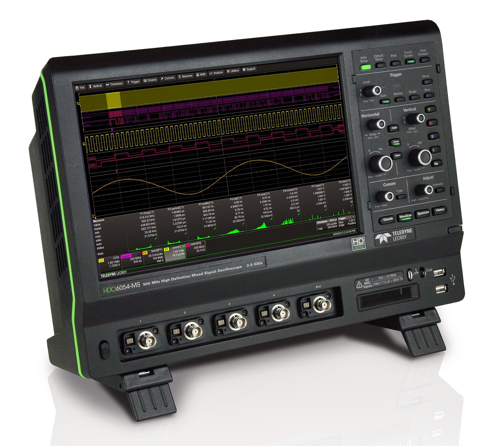Figure 1: An oscilloscope such as
Teledyne LeCroy's HDO6054-MS
serves a very broad range of
applications

Choosing an oscilloscope might seem to be a challenging task, but it doesn't have to be. Rather, it's a more-or-less logical process based on your measurement needs. Having said that, if the application for the instrument is "general lab work," the decision can become trickier.

Using Histograms (Part III)

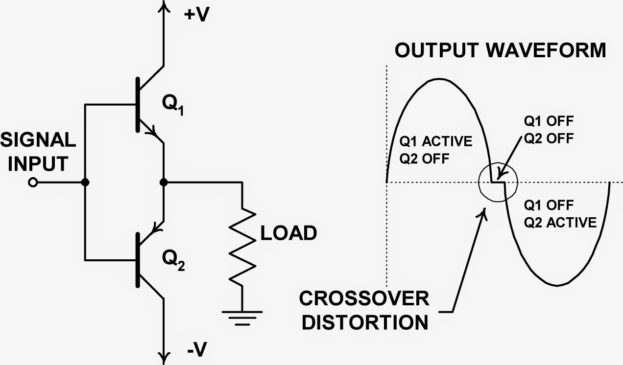Figure 1: A simplified view of a push-pull amplifier
showing the source of crossover distortion

In this third post in a series on using an oscilloscope's histogram capabilities, let's take a look at using histograms as a diagnostic tool. Diagnosing problems in a circuit calls for good skills and some intuition on top of good measurement tool. In general, though, the more ways in which you're able to look at a problem, the more likely it is that you'll turn up the root cause.

The History of Jitter (Part II)

Figure 1: An example of using histograms to plot
the statistical distribution of edge arrival times

Resuming our review of the history of jitter and the evolving response to it, we'd arrived at the late 1990s, when more sophisticated analysis methods were necessary to get a good handle on jitter. In particular, statistical analysis came onto the scene. Statistics are a great tool for analyzing phenomena such as jitter that change more as you look at them harder.

The History of Jitter

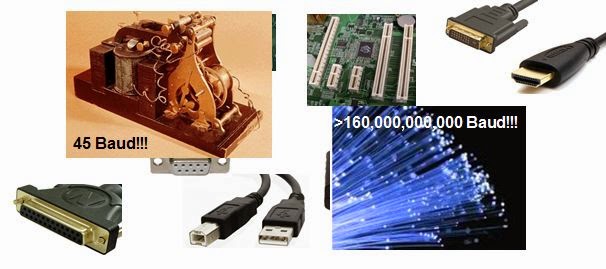Figure 1: The story of jitter spans 45-baud telegraph
machines to 160-Gbaud optical fiber

Jitter is a signal-integrity gremlin that's been with us for a long time. In fact, it's been with us since before anyone really needed to care about it. But as time has worn on, our perception of jitter has certainly changed, and with it our approaches to diagnosing it, measuring it, and ultimately dispatching it. Here, we'll begin a traversal of the "jitter story," surveying where we've been, where we are, and where we may be going in our dealings with the phenomenon.

Using Histograms (Part II)

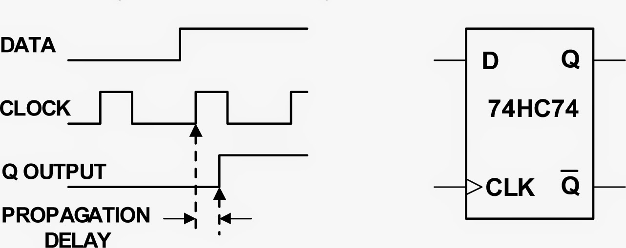Figure 1: A flip-flop's propagation delay is a typical spec

that can be derived using statistical analysis

In Part I of this series, we looked at some of the basics of histograms and how they can provide a statistical view into random variation of signal parameters. Next, let's look at how histograms can help us use statistical analysis to determine product specifications.

Using Histograms (Part I)

Figure 1: Histograms of the period, width, and
TIE show different distributions of time jitter

When we measure parameters of a waveform in a circuit or device, we rarely take a single measurement but rather a significant number of measurements. We want to see trends over time in the period, width, and time-interval error of a clock pulse, for example. Those parameters will have some nominal value, but there will typically be some random variation that we refer to as jitter.