The History of Jitter (Part II)

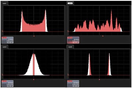
Figure 1: An example of using histograms to plot
the statistical distribution of edge arrival times

Resuming our review of the history of jitter and the evolving response to it, we'd arrived at the late 1990s, when more sophisticated analysis methods were necessary to get a good handle on jitter. In particular, statistical analysis came onto the scene. Statistics are a great tool for analyzing phenomena such as jitter that change more as you look at them harder.

A simple, yet telling, application of statistical analysis to the characterization of jitter would be to use histograms to compile a statistical distribution of edge arrival times (Figure 1). However, if we were to look at four different signals, we would see four different distributions. But those distributions all have at least one thing in common. If you look at the outside edges of each of the histograms, they all exhibit a similar shape. There's a "falling-off" shape to those edges that's half-Gaussian, or random, in character.

Figure 2: Jitter has two main components: random (in white
in all four histograms) and deterministic (in salmon)

Consider the histogram at the upper left of Figure 2 (or any of them, for that matter). What it reveals is that jitter has two broad components. Keep in mind what a histogram is: It shows us the shape of the statistical distribution of parameter values. So when we look at that upper-left display, what we see is that jitter has two parts. Those "falling-off" Gaussian tails at either end of the distribution, shown in white, represent the random component of jitter. This component of jitter is unbounded, so statistically speaking, the longer you measure, the larger it gets, because theoretically, an edge can arrive anywhere at any time.

The other component, seen in a salmon hue, is the deterministic component of jitter. This component determines the shape of the distribution between the two tails. Deterministic jitter is bounded, so assuming a sufficient sample size, that part of the distribution will not grow as you measure longer and longer.

Figure 3: Measuring peak-to-peak
jitter is a losing proposition

One question that often arises with regard to jitter measurement is, "why not just measure peak-to-peak jitter?" Recall that the random component of jitter is unbounded. Measurement of peak-to-peak values for anything unbounded is not a well-defined statistic. Thus, the expected peak-to-peak value will grow as the population increases (Figure 3). There can always be unrepresentative "outliers" in the distribution that further distort the results when measuring peak-to-peak jitter.

Well, then, what about measuring the standard deviation of jitter? Nope, that's not a very good idea either. The standard deviation of the distribution isn't going to be very meaningful if the distribution isn't Gaussian. You might see distributions with different shapes that have the same standard deviation. Thus, as a single figure of merit, standard deviation doesn't tell you very much.

So at the end of the day, it comes back to bit errors and the propensity of our system to generate them. If we look at enough bits, we are statistically guaranteed to see a bit error. By the late 1990s, what mattered was how many bit errors we expect to see for a given number of bits—the bit-error ratio (BER). If we get one bit error in one Mbit of data, that's a BER of 10^-6. The typical confidence level required by many serial-data standards is a BER of 10^-12. That's one bit error in 1000 Gbits of data, and that's a number that you hear a lot in conjunction with compliance testing.

The late 1990s saw a shift in emphasis to BER as a function of jitter. We'll turn our attention to that topic in our next installment in this informal survey of the history of jitter.