You need to test, we're here to help.

You need to test, we're here to help.

25 April 2022

Setting Up Your Oscilloscope for EFT Testing

Figure 1: The typical EFT test signal consists of multiple exponential pulses arranged as pulse bursts.
Figure 1: The typical EFT test signal consists of
multiple exponential pulses arranged as pulse bursts.
A third type of electromagnetic compatibility (EMC) testing deals with how devices respond to electrical fast transients (EFT). EFTs are a series of fast, high frequency pulses, often occurring in bursts. These transient events are the result of electrical arcing. EFT pulse bursts occur when a power connection is made or broken, equipment is powered down or circuit breakers are switched. They also occur when inductive loads such as relays, switch contactors or heavy-duty motors produce bursts of narrow high-frequency transients on the power distribution system when de-energized.

The typical compound waveform used for EFT testing is shown in Figure 1.

Figure 2: Acquisition of two EFT bursts at 1.25 GS/s, zoomed to show several timing epochs.
Figure 2: Acquisition of two EFT bursts at
1.25 GS/s, zoomed to show several timing epochs.
The pulse waveform for EFT testing is defined by a risetime of 5 ns and a pulse width of 50 ns. These pulses are combined into bursts of 5 to 50 pulses spaced at from 10 to 100 µs (10 to 100 kHz). The bursts are typically spaced as much as 300 ms apart. Figure 2 shows an EFT test signal, with two EFT bursts captured by an oscilloscope on channel 2 sampled at 1.25 GS/s.

The two EFT pulse burst are shown in the upper left-hand trace (the two pink blocks). A series of zoom-on-zoom traces are opened to show several timing epochs. Trace Z2 (second from top left) shows a single burst. The zooms keep expanding the horizontal scale until finally at Z8 (bottom right) we see a single EFT pulse.

Following are six, important things to do to make sure you get the best EFT test measurements from your oscilloscope.

18 April 2022

Setting Up Your Oscilloscope for Surge Testing

Figure 1: A typical EMC surge test waveform with 1.2 µs rise time and 50 µs half amplitude time. Zoom trace Z1 shows the details of the rise time. Click any image to expand it.
Figure 1: A typical EMC surge test waveform with
1.2 µs rise time and 50 µs half amplitude time.
Zoom trace Z1 shows the details of the rise time.
Click any image to expand it.
Electrical surges result from phenomena like lightning strikes and switching transients.  Electronic devices are subjected to simulated surges to confirm that they continue to operate properly following a surge, just as they are tested against electrostatic discharge. 

Surge pulses are similar to ESD pulses in that they have a very fast rise time, but the fall time is much, much slower. Figure 1 shows a typical surge pulse waveform. Surge testing involves similar measurements to those made for  ESD pulse testing—such as rise time, pulse width and max—but surge testing also requires some additional measurements, such as area under the pulse curve and transmitted charge. 

Figure 2: To verify the surge generator waveform, the oscilloscope is connected to the generator through an attenuator.
Figure 2: To verify the surge generator waveform, the
oscilloscope is connected to the generator through an attenuator.
As with ESD pulse tests, oscilloscopes are primarily used to “test the tester,” confirming the output of the surge generator. So, before a surge generator is hooked up to the device under test, it's required to hook it up to an oscilloscope and conduct a series of measurements to make sure the surge pulse is within specification. Figure 2 shows a typical surge test setup.

Following are three, important things to do to make sure you get the best surge measurements from your oscilloscope.

11 April 2022

Setting Up Your Oscilloscope for ESD Pulse Testing

Figure 1: An ESD calibration test setup.  The ESD gun discharges its waveform into a properly attenuated current target.
Figure 1: An ESD calibration test setup. 
The ESD gun discharges its waveform
into a properly attenuated current target. 
Electrostatic discharge (ESD) pulse tests are a type of conducted immunity testing done to confirm that a device can withstand a sudden transient electrostatic discharge. It is done by using an ESD gun to shoot a pulse of the required voltage at a device while testing that the DUT continues to operate properly. The ESD pulse shape simulates a person, carrying a static charge, touching a device. When their fingertip first touches the device, there is a leading edge with a high peak and fast decay, often visible in the real world as a spark flying from the fingertip. This is followed by a second edge due to the charge in the rest of the human body that propagates toward the fingertip with a time delay.

Oscilloscopes are most often used to “test the tester” in ESD pulse test setups, confirming that the pulse from the ESD gun is the right shape and meets the requirements of the standard to which the device is being tested. A typical calibration test setup is shown in Figure 1. The pulse from the ESD gun is fired directly into a current shunt target connected to the oscilloscope through an attenuator required to keep the signal within the limits of the oscilloscope’s 50 Ω input, which is used for this testing. Then, key parameters of the ESD pulse are measured per one of several standards, such as IEC 61000-4-2.  

ESD standards require a range of measurements. The most common are the initial edge 10% to 90% rise time, peak amplitude, pulse width, amplitude and current levels at specified times from the initial edge (e.g., T1 and T2), and time to half value. 

Following are four, important things to do to make sure you get the best ESD pulse measurements from your oscilloscope.

04 April 2022

Oscilloscope Basics: When to Use Trend to Graph Oscilloscope Measurements

Figure 1: Applying the Trend operator to the same input waveform illustrates how the Trend is asynchronous to the input waveform.
Figure 1: Applying the Trend operator to the
same input waveform illustrates how the
Trend is asynchronous to the input waveform.  
In a previous post, we described the characteristics of the Track math function and two key applications of using Tracks to graph oscilloscope measurement data: anomaly detection and waveform demodulation. In this post, we'll discuss the characteristics and uses of the Trend function.

To illustrate an important distinction between Tracks and Trends, the Trend math operator in Figure 1 is now applied to the same signal as was the Track in our previous post without first reacquiring the input waveform. 

Note that unlike a Track, the Trend is not time-synchronized to the input waveform. Only the order of events, and not the timing of events, is retained. The underlying shape of the Track may be displayed in the Trend because the same measurement values from a single acquisition are displayed in the same sequence—however, the timing information of when each of the values has occurred is not retained in the Trend. Therefore, unlike the Track, the Trend does not point to the location of an anomaly. Without time scaling, the Trend does not have the frequency information needed to demodulate an input waveform.

28 March 2022

Oscilloscope Basics: When to Use Track to Graph Oscilloscope Measurements

Figure 4: The Trend (green) retains a history of pulse widths, while the Track (blue) shows only a flat line corresponding to the most recent width.
Figure 1: Pulse Width Modulated waveform (yellow)
and Track math operator (blue),
where the X-axis scaling is identical for both.
Modern oscilloscopes contain many tools that can be used for analyzing data, including Track and Trend math functions. Both Tracks and Trends graphically display measurement results and locate anomalies. The main similarity between Tracks and Trends is that the Y-axis of both operators is the measurement parameter itself (for example, Pulse Width, Duty Cycle, Rise Time, Slew Rate, etc.). The main difference between the two math operators is their X-axis, in which the Track uses the identical X-axis and synchronous horizontal scaling as the input waveform, whereas the Trend uses units of chronology. A Track, in essence, is a waveform of the measurement values. A Trend is a data logger showing the history of change in measured parameter values, but points are not necessarily synchronous with the measured waveform.

Use Tracks for Anomaly Detection

The Track provides valuable debugging information by directly pointing to an area of interest. 

Notice the negative-going spike in the Track waveform in Figure 1. Figure 1 occurs at the point in time where the input waveform reaches its most narrow pulse width, and the Track instantly finds it, indicating when one measurement deviates from the others in the graph. The Track identifies the exact location in time where the narrowest or widest pulse width has occurred, and fully describes the measurement changes occurring throughout the entire waveform. Since oscilloscopes can acquire thousands or even millions of waveform edges within a single acquisition, the Track allows an engineer to quickly "find the needle in a haystack".

21 March 2022

PCI Express 4.0 Error Detection Using a BERT and Oscilloscope

Figure 1: BERT and Oscilloscope connection for PCI Express 4.0 error detection.
Figure 1: BERT and Oscilloscope connection
for PCI Express 4.0 error detection.
The PCI Express® 4.0 standard specification requires an oscilloscope with at least 25 GHz analog bandwidth and a BERT which can test bit rates of at least 16 Gbps. The BERT provides a known input pattern to the PCIe® device under test (DUT), and the DUT is instructed to regenerate the identical bit pattern while placed in loopback mode. Since a BERT can output a signal when a bit error is detected, this signal can be input to the oscilloscope to trigger a synchronized capture when an error occurs. By combining the capabilities of these two instruments, a powerful combination of real-time error detection and characterization can emerge.

Connecting the Instruments

In Figure 1, a known pattern is connected from the BERT PPG D1 output to the PCIe DUT input via a 2.92 mm K-type cable. The DUT attempts to regenerate the same data pattern, while the DUT output is routed to both the BERT error detector input and the oscilloscope channel 1 via 2.92 mm K-type tables and a power splitter. An error-free reference signal is connected between the BERT D2 output to the oscilloscope channel 2, along with the error trigger signal from the error detector output to the oscilloscope channel 3. An oscilloscope Edge trigger is set on the rising edge of the error detector output signal on C3.

14 March 2022

WavePulser 40iX vs. Time Domain Reflectomer (TDR) or Vector Network Analyzer (VNA)

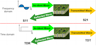
Figure 1: S-parameters and TDR responses are two means to the same end, characterizing interconnects.
Figure 1: S-parameters and TDR responses are two means to
the same end, characterizing interconnects.
Oscilloscopes are used to measure signals, usually as voltages vs. time, and signals come from active devices. But interconnects are passive structures that don’t produce their own signals. To characterize interconnects, you need a stimulus-response system.

There are two, principal types of stimulus-response systems used to characterize interconnects: Vector Network Analyzers (VNAs) used to measure S-parameters in the frequency domain, and Time Domain Reflectometers used to measure impulse responses in the time domain. Each uses a different type of incident signal and a different formalism, but as long as the interconnect is linear, passive and time invariant, both S-parameters and impulse responses yield the same information content in different formats and can be translated from one into another.

So, which do you need? We’ll look briefly at what each does and what are the criteria that might require you to have one versus the other.