USB4 Alt-Mode Testing: DPAUX and USB-PD

Figure 1: The interfaces that make up the USB-C connector and their relationships.

The USB Type-C® (USB-C) connector supports not only USB data transfers at speeds of up to 20 Gb/s but also can be reconfigured to support a wide variety of other interfaces through the USB4 provision for alternative (Alt) modes. The Alt-Mode protocols supported include Thunderbolt™, Mobile High-Definition Link (MHL), Peripheral Component Interconnect Express (PCIe®), High-Definition Multimedia interface (HDMI®) and DisplayPort™ (DP).

The diagram of the USB-C receptacle in Figure 1 shows where it potentially switches from normal operation into Alt-Mode.

Testing DisplayPort 2.0 vs. USB4 Over USB Type-C Connectors

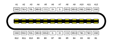Figure 1: The pin out of the USB Type-C connector.

DisplayPort™ 2.0 (DP 2.0) is a high-resolution video interface and USB4® is a high-speed data interface; what they have in common is the USB Type-C® (USB-C) connector. While DP 2.0 can also be deployed on the standard DisplayPort as well as mini-DisplayPort connectors, it is the USB-C connector that really excites electronics manufacturers because now they can use a single connector for high-speed data, high-resolution video and even power distribution. 

Figure 1 shows the pin assignments for a USB-C connector, which is a mechanically reversible connector that includes four, high-speed differential data lines: TX1, TX2, RX1 and RX2.

In USB4 operations, the four data lines TX1, TX2, RX1 and RX2 form a dual-lane, duplex signal path, supporting 10 and 20 Gb/s transfers on each line. When operating in USB4 Alt mode, up-to-four of these buses can be reassigned to become four DP 2.0 video lanes, which operate at 10, 13.5 or 20 Gb/s.

Testing for both interfaces over the USB-C connector is similar, but there are some notable differences.

DisplayPort 2.0 Physical Layer Testing

Figure 1. Functional diagram of DisplayPort 2.0
over USB-C Source (Tx) PHY testing.

The Video Electronics Standards Association (VESA) DisplayPort 2.0 video interface introduces a new performance standard with an increase in data bandwidth of three times compared to the older DisplayPort 1.4a specification, achieved by using four lanes of  up-to-20 Gb/s data per lane. This permits display resolutions to better than 8K, higher refresh rates and better dynamic range. These advantages are available using native DisplayPort connectors as well as the USB Type-C connector, which allows devices to handle video data, USB data and power all in the same connector.

With the USB-C cable now carrying DisplayPort and lower-speed sideband data, testing for USB devices has expanded to cover many dependencies between these protocols. This series will give an overview DisplayPort 2.0 physical-layer testing and how it relates to USB testing.

What Is Differential Manchester Encoding?

Figure 1. Differential Manchester encoding is based on the
presence or absence of a transition, whereas Manchester 
encoding relies on the polarity of the transition.

Differential Manchester Encoding (DME) is an example of a differential, bi-phase encoding technology. DME is specified in the IEEE 802.5 standard for Token Ring local area network (LAN) topology. 

Manchester is categorized as bi-phase encoding because the signal is checked twice every bit interval, also called self-clocking. Each check is one “tick”, each bit interval equals two ticks of the clock. This removes the need for the separate clock signal that is required for Non-Return to Zero (NRZ) encoding. Instead, data and clock signals are combined into a single, two-level, self-synchronizing data stream. The clock can be "extracted" by measuring the timing of the edges.

Figure 2. In Manchester encoding, the polarity of the
transition that occurs mid-interval determines the logic.

In Manchester encoding, we see a digital modulation scheme where voltage transitions rather than voltage levels are used to represent 1s and 0s. In IEEE 802.3 Manchester, a high-to-low transition occurring in the middle of the bit interval represents logical 0, while a low-to-high transition represents logical 1 (the G.E. Thomas variant reverses this logic). Significant transitions always occur in the middle of the bit interval to ensure clock synchronization. Transitions at the start of a period are only used to reset the polarity to achieve the proper transition for the next bit. This increases error detection capabilities, compared to NRZ, but also increases the bandwidth needed to transmit the signal at the same data rate, making it a better candidate for short-distance applications.

Figure 3. Even inverted, DME signals result in same logic.

The most prominent feature that distinguishes DME from classic Manchester encoding is that, in DME only the presence or absence of a transition during the bit interval is important, not the polarity. The presence of a transition represents a logical 0, while the absence of a transition represents a logical 1. Whether the signal goes line-high or line-low depends simply on its state the previous bit interval. This increases bit rate at lower bandwidths, because one bit is guaranteed to occur every interval. It also helps with data recovery in noisy environments, like automotive, because DME allows for a data stream to be inverted, yet still be properly decoded, unlike classic Manchester where the polarity is significant. 

DME is used for 10Base-T1S Automotive Ethernet, a short-distance, low-bandwidth application with either a point-to-point or bus topology up to 25 m. 

Teledyne LeCroy offers QualiPHY compliance test solutions for 10Base-T1S, including a QPHY-10Base-T1-TDR option that automates all required MDI S-parameter tests using the WavePulser 40iX.

For more information about 10Base-T1S compliance testing, see the on-demand webinar, How to Become an Expert in Automotive Ethernet Testing, Part 1.

See also:

Automotive Ethernet MDI S-parameter Testing

Automotive Ethernet in the Vehicle

Fundamentals of Automotive Ethernet

Using Tracks to Demodulate Frequency/Phase Modulated Signals

Figure 1: A low-pass filtered track of the Frequency
measurement demodulates the linear frequency
sweep in a radar chirp. The frequency domain
FFT shows the range of the frequency change.

If you are involved in RF measurements, you will eventually need to demodulate a signal. Angle modulation of either phase or frequency are the most commonly encountered modulation types. The Frequency measurement is an all-instance timing parameter that measures the frequency of every cycle in an acquired waveform. Similarly, Time Interval Error (TIE) measures the instantaneous phase of a signal on a cycle-by-cycle basis. Track functions of these measurements, which plot the values of the measurement parameter versus time, are useful for demodulating frequency and phase modulated signals, as shown in the examples below.

Finding “Unknown” Waveform Anomalies

Figure 1: Width “exclusion” trigger captures
pulse widths outside the range of 980 ns to 1 µs.
The first anomaly captured is a width of 2.99 µs.

Using SmartTriggers® and statistics to find waveform anomalies is easy if you know the characteristics of the anomaly, but how do you find intermittent, anomalous events when you don’t know what you’re looking for? The answer: start with what you do know!  

Look for What’s “Not Normal”

A simple approach is to measure the nominal waveform, then trigger the oscilloscope on waveform elements that differ from nominal. Figure 1 shows a 500 kHz square wave with a roughly 50% duty cycle, so the pulse width is normally about 1 µs (the Width measurement shows a mean of 997 ns). This nominal width does not change significantly with any regularity and gives us a basis on which to begin looking for anomalies.

Finding Intermittent Events

Figure 1: Statistics for 1261 Width measurements
taken over 97 acquisitions on the Measure table.
Width statistics can help determine the set up
of a Glitch SmartTrigger.

Glitches, dropouts, runts, aperiodicity, missed cycles, slow edges—whatever you call them, they are irregular waveform elements that can wreak havoc with you circuit operation. Because they do not occur with regularity, they can be hard to find and correlate with whatever synchronous events may be causing them. How can you use your oscilloscope to easily find intermittent events where they occur? The answer is by judicious application of the oscilloscope’s measurement statistics and SmartTriggers®.