Use Trend Functions To Take Power's Pulse

When troubleshooting or debugging almost anything, the first step is usually to check what's going into the device or circuit and what's coming out on the other side. So it is with power supplies, which leads us to power line monitoring and trend functions.

Most modern digital oscilloscopes provide a Trend function, as do most Teledyne LeCroy instruments. For power line monitoring, as well as any measurement in which you're interested in seeing how parameters change over time, the Trend function is a great tool.

Basically, the Trend function creates a waveform out of a series of parameter measurements values presented in the order they were taken. You can create a Trend plot of up to 1 million measurement values, which ought to be enough to give you an idea of how any parameter is changing over time.

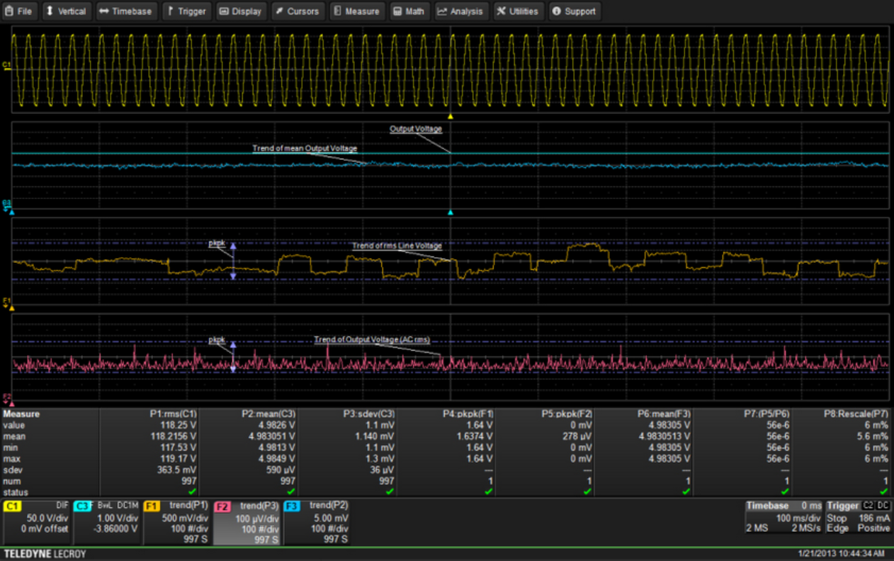
Figure 1: Trend plots of line voltage and power supply
outputs.

Let's look at a power supply test in which the input line and output voltages are monitored (Figure 1). Here, the AC line input is acquired on Channel 1 (top trace) using a differential probe. Channel 3 is the DC output of the power supply. For each measurement, the record length is one second.

Three parameters are being measured: parameter P1 is the RMS value of the power line. Parameter P2 is the mean value of the DC output voltage. Parameter P3 is the standard deviation (ACrms) value of the power supply's output. This is used to monitor small changes in the power supply's output level including ripple and line-related output changes.

Function trace F1 is a trend plot of the AC input voltage, showing the RMS line voltage over 1000 acquisitions (about 17 minutes). Similarly, function trace F2 shows the trend plot of P3 (standard deviation) taken at the same time. Function trace F3 is a trend plot of the mean output voltage, also taken together with F1 and F2.

The trend plot of the line voltage shows variations of about 1.6 V over the 17-minute measurement span as read by parameter P4 (peak-to-peak voltage of F1). Meanwhile, the AC variation of the power supply output is 278 μV. The mean power-supply output (P6) is 4.98 V.

So what have we learned about our line voltage and power-supply output? A visual comparison of the trend plots of the line-voltage variations with either the mean power-supply output or the AC variation of the output reveals no apparent relationship. Thus, the power supply seems to have good line regulation. Using the measurements that have been taken, we can also compute the line regulation. Parameter P7 uses parameter math to take the ratio of the peak-to-peak output variation divided by the mean output voltage. P8 rescales this to a percentage, again using parameter math, by multiplying by 100 and changing the units to percent. Thus, the line regulation is 0.0056%.

On Teledyne LeCroy oscilloscopes, trend functions can be set up from the parameter setup dialog box or from the Math setup dialog box. Any parameter measurement can be the source of a trend plot, with the number of values in the plot ranging from two to 1 million (depending on the oscilloscope model). Scaling may be set automatically or manually. Note that trend functions can be manipulated like any other waveform by applying math operations or parameter measurements.