Filtering Signals with MATLAB

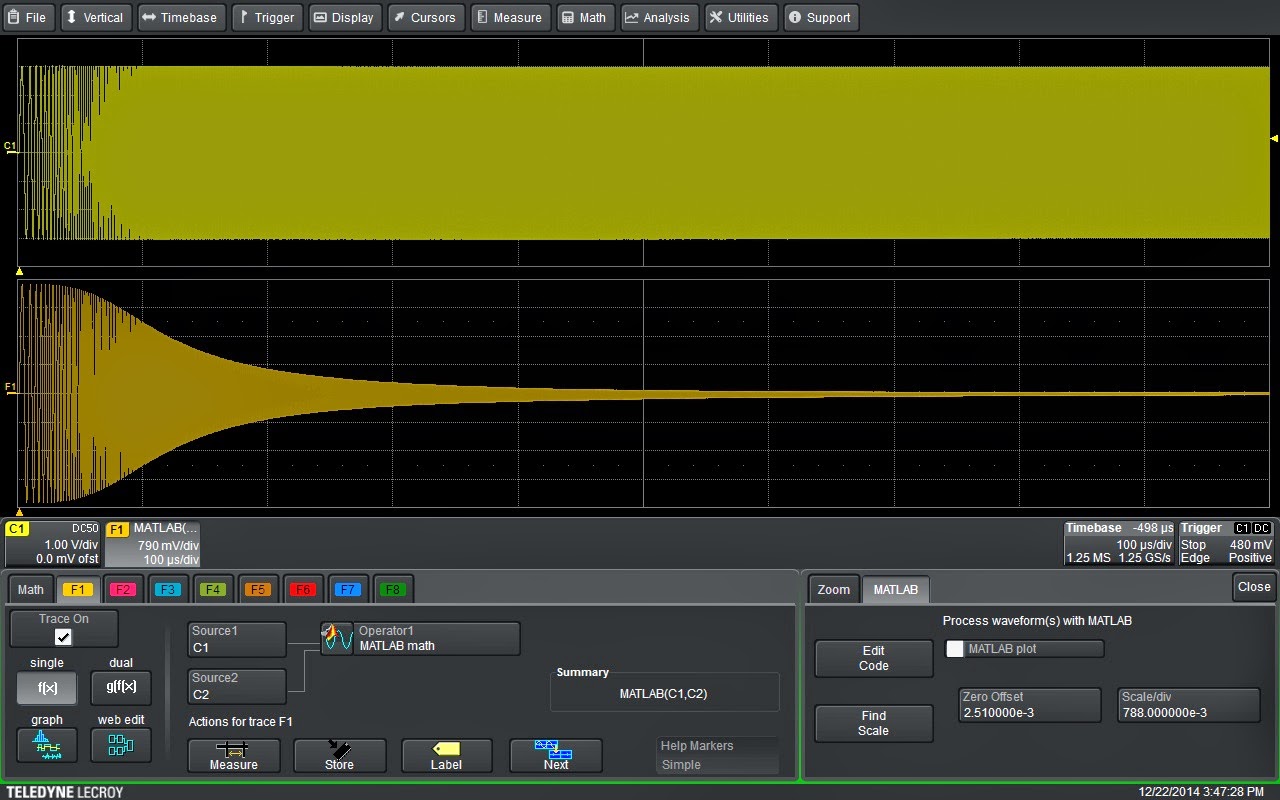
Figure 1: A 2-pole, 1-MHz Butterworth low-pass filter
applied to an acquired waveform

Touted by its maker as "the language of technical computing," The MathWorks' MATLAB is a veritable Swiss Army knife for engineers, scientists, and perhaps anyone involved in technical endeavors. MATLAB serves a myriad of applications in programming, data analysis, application development, modeling and simulation, and... wait for it... instrument control!

With MATLAB, you can make Teledyne LeCroy's oscilloscopes jump through all sorts of hoops. You can run it on most Windows-based instruments and live-stream acquired data into MATLAB for processing and/or analysis, and then stream that data right back into the oscilloscope for further processing and/or display. It can also be used to create custom math or measurement algorithms to make non-standard measurements or filter and process signals.

Let's take a look at an example of the latter case. Often, you'll find a need to filter a signal before analysis. It might be a matter of equalizing the frequency response, or perhaps noise reduction. No matter what the reason, MATLAB provides a very handy way to embed a user-defined filter in the oscilloscope's processing path.

MATLAB comes with a number of filter types; The MathWorks offers lots of online resources to get you started in filter design and implementation as well. Figure 1 shows an example of a 2-pole, 1-MHz Butterworth low-pass filter applied to an acquired waveform using the oscilloscope's MATLAB math function.

Figure 2: A view of the built-in editing window
in the HDO6000's MATLAB Math function

The MATLAB math function allow users to call the MATLAB program and execute a script file directly in the oscilloscope's processing path. The output from MATLAB is returned to the next processing stage and normal oscilloscope operation ensues. In Figure 1, we show the basic setup of the MATLAB math function on an HDO6000 oscilloscope. The function accepts one or two input signals and returns a single output. Selecting the MATLAB tab in the instrument's Math dialog box allows users to load an existing MATLAB (.m) file or create a new one in the built-in editor (Figure 2).

The .m file used in this example is shown in Figure 3. This code implements the 2-pole, 1-MHz Butterworth low-pass filter applied to the signal in Figure 1. The filter used here is a relatively slow cutoff, second-order filter. The command to create the filter coefficients is in the next-to-last line of code, where b represents the numerator coefficients of the digital filter and a represents the denominator coefficients of the digital filter.

Figure 3: The MATLAB .m code that implements a 2-pole, 1-MHz
Butterworth low-pass filter applied to the signal in Figure 2

The arguments for the Butterworth filter are order (2 in this case) and the cutoff frequency, which must be normalized to Nyquist. That's why we have divided by half of the sampling frequency, Fs.

The filter is implemented using the filter command in the final line of code, which applies the filter coefficients to the selected data. In this case, that is the input waveform, WformIn1). The commands in the first five lines of code queries the oscilloscope via Microsoft automation to obtain the sampling frequency.

In this example, we've implemented a simple low-pass filter. But this concept can be extended for use with any of the available MATLAB functions or scripts. Try a few ideas of your own and see how the power of MATLAB can be applied to the filtering of live signal acquisitions.