![]() |
| Figure 1: The typical EFT test signal consists of multiple exponential pulses arranged as pulse bursts. |
![]() |
| Figure 2: Acquisition of two EFT bursts at 1.25 GS/s, zoomed to show several timing epochs. |
![]() |
| Figure 1: The typical EFT test signal consists of multiple exponential pulses arranged as pulse bursts. |
![]() |
| Figure 2: Acquisition of two EFT bursts at 1.25 GS/s, zoomed to show several timing epochs. |
![]() |
| Figure 1: A typical EMC surge test waveform with 1.2 µs rise time and 50 µs half amplitude time. Zoom trace Z1 shows the details of the rise time. Click any image to expand it. |
Surge pulses are similar to ESD pulses in that they have a very fast rise time, but the fall time is much, much slower. Figure 1 shows a typical surge pulse waveform. Surge testing involves similar measurements to those made for ESD pulse testing—such as rise time, pulse width and max—but surge testing also requires some additional measurements, such as area under the pulse curve and transmitted charge.
![]() |
| Figure 2: To verify the surge generator waveform, the oscilloscope is connected to the generator through an attenuator. |
Following are three, important things to do to make sure you get the best surge measurements from your oscilloscope.
![]() |
| Figure 1: An ESD calibration test setup. The ESD gun discharges its waveform into a properly attenuated current target. |
Oscilloscopes are most often used to “test the tester” in ESD pulse test setups, confirming that the pulse from the ESD gun is the right shape and meets the requirements of the standard to which the device is being tested. A typical calibration test setup is shown in Figure 1. The pulse from the ESD gun is fired directly into a current shunt target connected to the oscilloscope through an attenuator required to keep the signal within the limits of the oscilloscope’s 50 Ω input, which is used for this testing. Then, key parameters of the ESD pulse are measured per one of several standards, such as IEC 61000-4-2.
ESD standards require a range of measurements. The most common are the initial edge 10% to 90% rise time, peak amplitude, pulse width, amplitude and current levels at specified times from the initial edge (e.g., T1 and T2), and time to half value.
Following are four, important things to do to make sure you get the best ESD pulse measurements from your oscilloscope.
![]() |
| Figure 1: Applying the Trend operator to the same input waveform illustrates how the Trend is asynchronous to the input waveform. |
To illustrate an important distinction between Tracks and Trends, the Trend math operator in Figure 1 is now applied to the same signal as was the Track in our previous post without first reacquiring the input waveform.
Note that unlike a Track, the Trend is not time-synchronized to the input waveform. Only the order of events, and not the timing of events, is retained. The underlying shape of the Track may be displayed in the Trend because the same measurement values from a single acquisition are displayed in the same sequence—however, the timing information of when each of the values has occurred is not retained in the Trend. Therefore, unlike the Track, the Trend does not point to the location of an anomaly. Without time scaling, the Trend does not have the frequency information needed to demodulate an input waveform.
![]() |
| Figure 1: Pulse Width Modulated waveform (yellow) and Track math operator (blue), where the X-axis scaling is identical for both. |
The Track provides valuable debugging information by directly pointing to an area of interest.
Notice the negative-going spike in the Track waveform in Figure 1. Figure 1 occurs at the point in time where the input waveform reaches its most narrow pulse width, and the Track instantly finds it, indicating when one measurement deviates from the others in the graph. The Track identifies the exact location in time where the narrowest or widest pulse width has occurred, and fully describes the measurement changes occurring throughout the entire waveform. Since oscilloscopes can acquire thousands or even millions of waveform edges within a single acquisition, the Track allows an engineer to quickly "find the needle in a haystack".
![]() |
| Figure 1: BERT and Oscilloscope connection for PCI Express 4.0 error detection. |
In Figure 1, a known pattern is connected from the BERT PPG D1 output to the PCIe DUT input via a 2.92 mm K-type cable. The DUT attempts to regenerate the same data pattern, while the DUT output is routed to both the BERT error detector input and the oscilloscope channel 1 via 2.92 mm K-type tables and a power splitter. An error-free reference signal is connected between the BERT D2 output to the oscilloscope channel 2, along with the error trigger signal from the error detector output to the oscilloscope channel 3. An oscilloscope Edge trigger is set on the rising edge of the error detector output signal on C3.
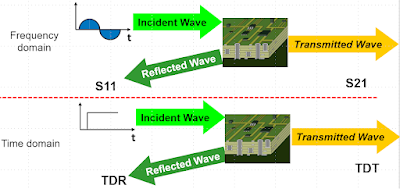
| Figure 1: S-parameters and TDR responses are two means to the same end, characterizing interconnects. |
There are two, principal types of stimulus-response systems used to characterize interconnects: Vector Network Analyzers (VNAs) used to measure S-parameters in the frequency domain, and Time Domain Reflectometers used to measure impulse responses in the time domain. Each uses a different type of incident signal and a different formalism, but as long as the interconnect is linear, passive and time invariant, both S-parameters and impulse responses yield the same information content in different formats and can be translated from one into another.
So, which do you need? We’ll look briefly at what each does and what are the criteria that might require you to have one versus the other.